3.1 Aggregate Demand

• Aggregate demand (AD) - The inverse relationship between all spending on domestic output and the aggregate price level of that output.

Components of AD

• Demand in the macroeconomy comes from four general sources, which are used to calculate the real GDP.

• AD measures the sum of consumption spending by households, investment spending by firms, government purchases of goods and services, and net exports (exports minus imports).

The shape of AD

General groups of substitutes for national output

• Foreign sector substitution effect - Goods and services produced in other nations.

  • Ex. →When the price of U.S. output increases, consumers begin to look for similar items produced elsewhere. A Japanese computer, a German car, and a Mexican textile all begin to look more attractive when inflation heats up in the United States. The resulting increase in imports pushes real GDP down at a higher price level.

• Interest rate effect - Goods and services in the future.

  • Ex.→ When more and more households seek loans, the real interest rate begins to rise, and this increases the cost of borrowing. Firms postpone their investment in plant and equipment, and households postpone their consumption of more expensive items for a future when their spending might go further and borrowing might be more affordable. This wait-and-see mentality reduces the current consumption of domestic production as the price level rises and real GDP falls.

• Wealth effect - Money and financial assets.

  • Wealth is the value of accumulated assets like stocks, bonds, savings, and cash on hand.

  • As the aggregate price level rises, the purchasing power of wealth and savings begins to fall. Higher prices, therefore, tend to reduce the quantity of domestic output purchased.

The AD Curve

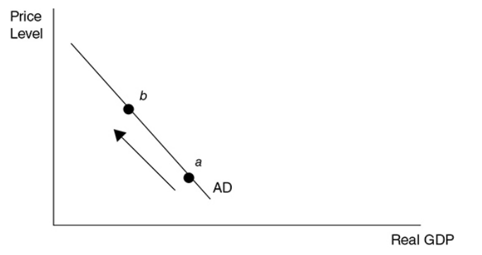
• The combination of the foreign sector substitution, interest rate, and wealth effects predicts a downward-sloping AD curve.

  • As the aggregate price level rises, consumption of domestic output (real GDP) falls along the AD curve. (This is the movement from a to b).

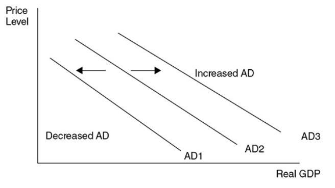
Changes in AD

• Since AD is the sum of the four components of domestic spending [C, I, G, (X — M)], if any of these components increases, holding the price level constant, AD increases, which increases real GDP. This is seen as a shift to the right of AD.

• If any of these components decreases, holding the price level constant, AD decreases, which decreases real GDP. This is seen as a shift to the left of AD.

  

• If you want to stimulate real GDP and lower unemployment, you need to boost any or all of the components of AD.

• If you feel AD must slow down, you need to rein in the components of AD.

Components of AD

• Consumer Spending (C) - If you put more money in the pockets of households, it is expected that they consume a great deal of it and save the rest. Consumers also increase their consumption if they are optimistic about the future.

• Investment Spending (I) - Firms increase investment if they believe the investment will be profitable. This expected return on the investment is increased if investors are optimistic about future profitability or if the necessary borrowing can be done at a low rate of interest.

• Government Spending (G) - The government injects money into the economy by spending more on goods and services, by reducing taxes, or by increasing transfer payments.

  • Government spending on goods and services is a direct increase in AD.

  • Lowering taxes and increasing transfer payments increase AD through consumer spending by increasing disposable income.

• Net Exports ( X - M) - When sales to foreign consumers are high and purchases from foreign producers are low, the net exports increase.

  • Foreign incomes - Exports increase with strong foreign economies. When foreign consumers have more disposable income, this increases the AD in the United States because those consumers spend some of that income on U.S.-made goods.

  • Consumer tastes - If American blue jeans become more popular in France, American AD increases. If French wines become more preferred by American consumers, AD in France increases.

  • Exchange rates - Imports decrease when the exchange rate between the dollar and foreign currency falls. This makes foreign goods to be more expensive causing consumers to buy fewer foreign-produced items.

3.2 Spending and Tax Multipliers

Multipliers

• Multiplier effect—The idea that an initial change in spending will set off a spending chain that is magnified in the economy.

• Marginal propensity to consume (MPC)—How much people consume rather than save when there is a change in income. This can also be explained as the portion of each new dollar of disposable income that consumers will spend rather than save.

• Marginal propensity to save (MPS)—How much people save rather than consume when there is a change in income. This can also be explained as the portion of each new dollar of disposable income that consumers will save rather than spend.

MPC and MPS

• Marginal Propensity to Consume (MPC) is calculated by dividing the change in consumption by dividing the change in disposable income.

• Marginal Propensity to Save (MPS) is calculated by dividing the change in savings by dividing the change in disposable income.

• MPC + MPS = 1

Spending Multiplier

• The spending multiplier, or fiscal multiplier, is an economic measure of the effect that a change in government spending and investment has on the Gross Domestic Product of a country. In other words, it measures how GDP increases or decreases when the government increases or decreases spending in the economy.

• Example: Matthew is an economist in the Federal Reserve, and he has been tasked with figuring out the ideal stimulus would be to increase GDP by $5,000,000. He reasons that in order to do that, he needs to figure out how much of their income consumers spend, and how much they save. Through looking at the market and statistical data, he sees that consumers are saving 35% of their after-tax income while spending 65% of it.

  • Using the spending multiplier formula (1 / MPS), he calculates that the Federal Reserve needs to inject (5,000,000 / 2.86) = $1,748,251.75 into the economy based on the current MPS.

  • Why does the government only have to spend $1.7M to increase GDP by $5M? This is because of the multiplier effect. One group of consumers consumes 65% of its new money on goods produced by another consumer. This consumer now has new money and consumes 65% of it on goods produced by someone else and so on.

  • Thus, consumers immediately consume 65 percent of this increase ($1.7M x .65). This $1.1M of consumption then triggers another line of consumption where these consumers consumer 65% of their earnings ( .65 x .65 x $1.7M). This goes on and on resulting in a multiple of 2.86.

  • The Spending Multiplier is largely related to how much consumers save, so if they save only 20% of their income and spend the rest, then whatever stimulus the Fed provides is magnified by 5 (1 / (0.2) = 5). This is the reason governments encourage spending during recessions. It can stimulate the economy and increase the flow of money.

Tax Multiplier

• The tax multiplier is used to determine the maximum change in spending when the government either increases or decreases taxes.

• The tax multiplier is basically the opposite of spending multipliers. It talks about how much people will not spend if taxes increase. If our net worth decreases because of taxes, it's natural for people to cut back on spending right?

  • The formula for this multiplier is -MPC/MPS. The tax multiplier will always be less than the spending multiplier. When spending occurs, we know that all of this money will be multiplied in the economy. But, when taxes are increased or decreased, not all the money received goes back into the economy. For example, if the government decreases taxes which gives individuals more disposable income, there is no guarantee they are going to spend all of the additional income.

  • Let's look at how we calculate this. If the MPC is 0.8 and the government imposes a $50 increase in taxes, what is the tax multiplier and what happened to the GDP?

    tax multiplier = -MPC/MPS

    tax multiplier = -0.8/0.2

    tax multiplier = -4

    GDP change: -4 * $50 = -$200

• One fun thing about tax multipliers is the fact that tax multipliers are smaller than spending multipliers. This is because spending multipliers have an immediate impact on the economy, but tax multipliers first have to go through someone's income before having an impact on the economy.

3.3 Short-Run Aggregate Supply (SRAS)

Aggregate supply (AS)

• The relationship between the aggregated price level of all domestic output and the level of domestic output produced.

Short-Run Aggregate supply (SRAS)

• The positive relationship between the level of domestic output produced and the aggregate price level of that output.

Macroeconomic Short Run

• In the macroeconomic short-run period, the prices of goods and services are changing in their respective markets, but input prices have not been adjusted to those product market changes. In the short run, the SRAS curve is typically drawn as upward sloping.

  

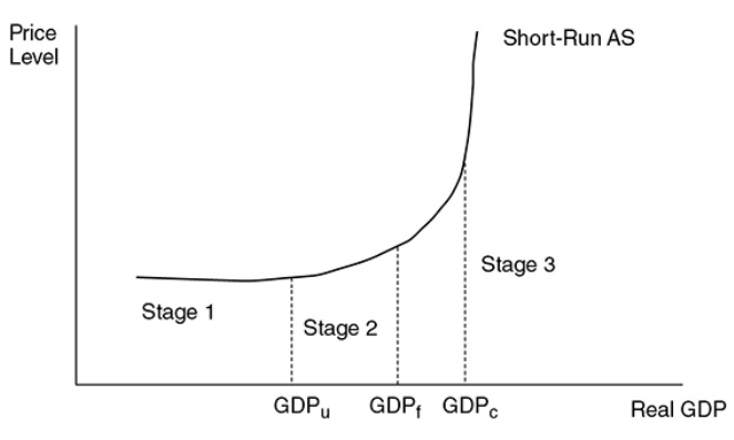
• In stage 1, the economy is in a recession with low production meaning they are many unemployed resources.

• In stage 2, real GDP increases and approaches full employment, available resources are harder to find and input costs begin to rise. If the price level for output rises faster than the rising costs, producers have a profit incentive to increase production.

• In stage 3, the AS curve is almost vertical, meaning that the economy is growing and approaching the nation’s productive capacity where firms cannot find unemployed units.

  • GDPu - Low production

  • GDPf - Full employment

  • GDPc - Nation’s productive capacity

Changes in AS

• In the short run, AS fluctuates without affecting the level of full employment.

Short-Run Shifts

• The most common factor that affects short-run AS → An economy-wide change in input (or factor) prices.

  • Input prices - If input prices fall economy-wide, the short-run AS curve increases without changing the level of full employment.

  • Tax policy - Some taxes are aimed at producers rather than consumers. If these “supply-side taxes” are lowered, short-run AS shifts to the right.

  • Deregulation - When the regulation of industries restricts their ability to produce, the short-run AS likely increases.

  • Political or environmental phenomena - For a nation as large as the United States, wars and natural disasters can decrease the short-run AS without permanently decreasing the level of full employment. For a smaller nation or a large nation hit by an epic disaster, this could be a permanent decrease in the ability to produce.

3.4 Long-Run Aggregate Supply (LRAS)

Long-Run Aggregate supply (LRAS)

• It is defined as the number of goods and services that an economy is capable of producing with the full employment of resources.

Macroeconomic Long Run

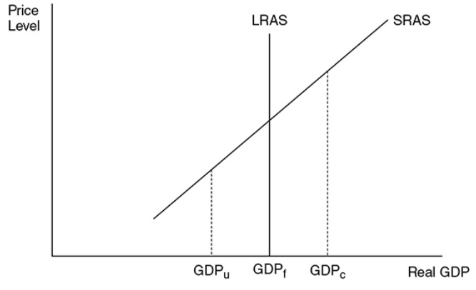
• In the macroeconomic long run, the input prices have enough time to fully adjust to market forces. Here all product and input markets are balanced, and the economy is at full employment (GDPf).

• The Classical school of economics asserts that the economy always gravitates toward full employment, so a cornerstone of classical macroeconomics is a vertical AS curve.

  

Long-Run Shifts

• Availability of resources - A larger labor force, a larger stock of capital, or more widely available natural resources can increase the level of full employment.

• Technology and productivity - Better technology raises the productivity of both capital and labor. A more highly trained or educated populace increases the productivity of the labor force.

• Policy incentives - If the policy provides large incentives to quickly find a job, full-employment real GDP rises. If the government gives tax incentives to invest in capital or technology, GDPf rises.

  • Ex. → Since the 1990s, the U.S. economy has seen dramatic increases in technology and investment in capital stock. This period produced a significant increase in the real GDP at full employment.

    

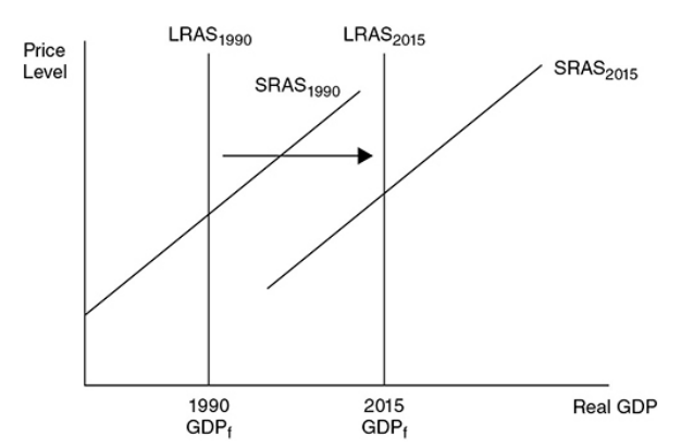
• When the LRAS curve shifts to the right, it indicates economic growth.

3.5 Equilibrium in Aggregate Demand-Aggregate Supply (AD-AS) Model

Equilibrium Real GDP and Price Level

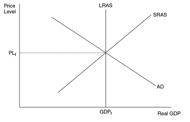
• Macroeconomic equilibrium - Occurs when the quantity of real output demanded is equal to the quantity of real output supplied. Graphically this is at the intersection of AD and SRAS. Equilibrium can exist at, above, or below full employment.

  

Recessionary and Inflationary Gaps

• Recessionary gap - The amount by which full-employment GDP exceeds equilibrium GDP.

  

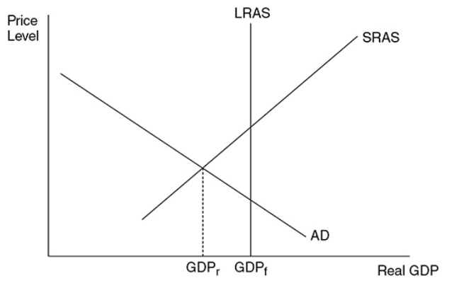
• In this picture, the recessionary gap is the difference between GDPf and GDPr, or the amount that the current real GDP must rise to reach GDPf.

• Inflationary gap - The amount by which equilibrium GDP exceeds full employment GDP.

  

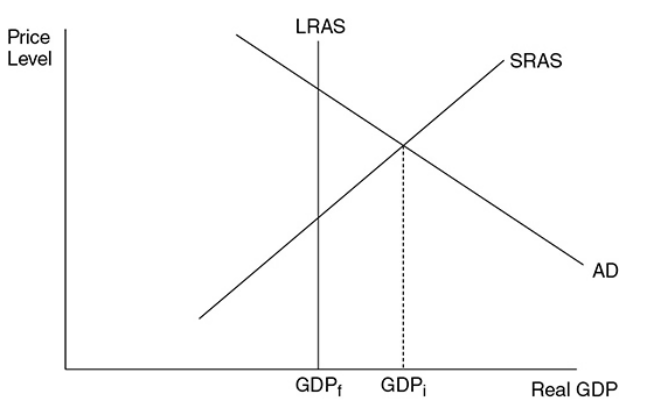
• In this picture, the inflationary gap is the difference between GDPi and GDPf, or the amount that real GDP must fall to reach GDPf.

3.6 Changes in the AD-AS Model in the Short Run

GDP Determinants

• Consumer spending

• Investment spending

• Government spending

• Net exports (exports-imports)

Supply Shocks

• Supply shocks - An economy-wide phenomenon that affects the costs of firms and the position of the SRAS curve, either positively or negatively. The shifts in SRAS are caused by these.

  

• Positive supply shocks might be the result of higher productivity or lower energy prices.

• Negative supply shocks usually occur when economy-wide input prices suddenly increase. Ex. → The Gulf War of 1990 to 1991.

3.7 Long-Run Self-Adjustment

Adjustment to a Recessionary Gap

• Based on this graph, the economy is currently operating at full employment. If consumers and firms begin to lose confidence in the labor market and overall economy, AD shifts to the left.

  • In the short run, this causes a recessionary gap as real GDP falls to GDPr meaning that unemployment rises and aggregate price levels fall from PL1 to PL2.

  • NOTE - One of the hallmarks of a recession is a decreased demand for many factors of production.

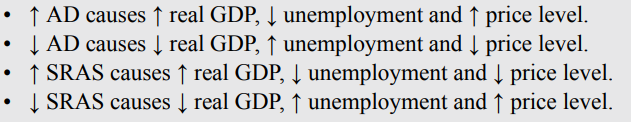
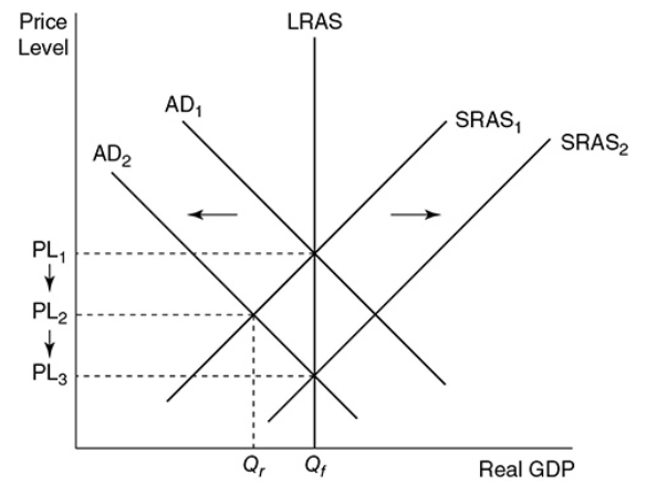
  • This recessionary gap fixes itself since the prices of the products will decrease, causing a gradual rightward shift of the SRAS curve to SRAS2. The curve shifts to the right until the gap is closed and the economy is back at GDPf.

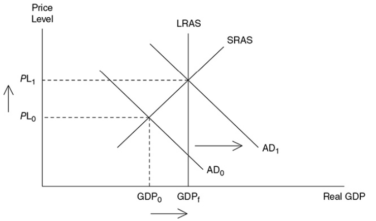
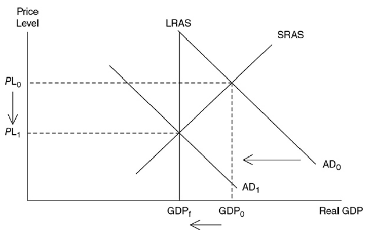
Adjustment to an Inflationary Gap

• When the AD curve increases, an inflationary gap happens to cause an increase in real GDP to GDPi (lower unemployment rate) and an increase in the aggregate price level to PL2.

  • When this happens, there’s stronger demand for labor and all of the other factors of production causing factor prices to rise. As the factor prices rise, the SRAS curve shifts to the left to SRAS2 eventually eliminating the inflationary gap, but at a higher aggregate price level of PL3.

3.8 Fiscal Policy

Expansionary Fiscal Policy

• Fiscal policy - Deliberate changes in government spending and net tax collection affect economic output, unemployment, and the price level. Fiscal policy is typically designed to manipulate AD to “fix” the economy.

• Expansionary fiscal policy - Real GDP is low and unemploymentis high when the economy suffers a recession. In the AD and AS model, there’s a recessionary equilibrium located below full ememployment

  

• If the government increases the spending or lowers net taxes, the AD curve increases. If taxes are lowered, the multiplier is smaller so to have the same increase in real GDP, the amount of taxes cut has to be larger than an increase in government spending.

• To resume, expansionary fiscal policy is the increases in government spending or lower net taxes meant to shift AD to the right.

Contractionary Fiscal Policy

• Contractionary fiscal policy - When the economy operates beyond full employement, inflation becomes a problem, so the government might need to contract the economy. This inflationary equilibrium is beyond full employement. It can be done by decreasing government spending or increasing net taxes, opposite to expansionary fiscal policy. Both of these options causes the AD to shift to the left with the purpose of decreasing real GDP and decreasing inflation.

  

• To resume, contractionary fiscal policy decreases government spending or increases net taxes to shift AD to the left.

• Sticky prices - If price levels do not change, especially downward, with changes in AD, then prices are thought of as sticky or inflexible. Keynesians believe the price level does not usually fall with contractionary policy.

  • On the other hand, Classical school economists believe that the long-run economy adjusts naturally to full ememploymentso they see the AS curve vertical. This implies that prices are flexible and can rise and fall, as seen in the last graph.

Short-Run Effects

• Lags and delays can sometimes occur with the discretionary fiscal policy.

• Non-discretionary fiscal policy refers to permanent spending or taxation laws already on books that help regulate the economy.

Calculating Fiscal Policies

• For government to help this economy correct itself back to the long-run:

  • to decide the amount of adjustment in taxes

  • goal: to shift aggregate demand to right in doing it back to where it connects SRAS AND LRAS at same GDP level.

• If we said that the MPC was .5, then that means that the MPS is also .5. If you remember from section 3.2, MPC + MPS always equals 1. The spending multiplier is calculated by dividing 1/MPS. So in this particular situation, the spending multiplier would be 2. This means that for every dollar the government spends, it will multiply twice in the economy. Since there is a gap of $50 billion than the governmthencould correct this economy by spending $25 billion.

  Since the MPC is .5, we would calculate the tax multiplier as .5/.5 (MPC/MPS). This would make the tax multiplier 1. So in order to correct this particular economy, the government would have to decreases taxes by $50 billion (the entire value of the gap).

3.9 Automatic Stabilizers

Automatic Stabilizers

• A type of fiscal policy that is already in place to offset the fluctuations or economic activity in our economy.

• It is typically used to counter the effects of negative supply shocks or recessions.

• Do not prevent anything.

• Income taxes and anti-poverty programs are examples of automatic stabilizers during an economic boom or recession.

Recessionary Period

• During a recession, less people are employed and less income is made for those unemployed families.

• If people have less money, they will spend less, worsening the economy.

• Programs like TANF (Temporary aid to needy families) will come to rescue.

• When more people are unemployed, more people will qualify for TANF, and more people will receive money from the government. This will, in turn, increase temporary "income" for the unemployed families, and they'll likely spend more. This will help the economy regain its strength with the help of increased spending.

• When the economy is improved, fewer families will qualify for TANF, which will lead to the size of the program decreasing. Less families will receive aid through TANF, so that the government is not always spending money.

Inflationary Period

• When inflation is rapidly increasing, income taxes will kick into effect. During the economic boom, the problem is that too many people are spending way too much.

• The government's income taxes can soothe this boom a little.

• Progressive income taxes describe income taxes that tax more if that household earns more income.