AP Macroeconomics Ultimate Guide
%%Unit 1: Basic Economic Concepts%%
Let’s have a quick overview of what economics is all about!
Economics
The study of how people, firms, and societies use their scarce productive resources to best satisfy their unlimited material wants.
It is the systematic study of choice.
In the realm of economics, all resources around us are considered to be limited; even the most basic things which exist around us like air or water.
</p>
Now, having an overall idea of what economics is all about. It’s time to dive into some crucial concepts:
1.1 Scarcity
- All factors of production are scarce; therefore, the production of goods and service are also scarce.
- The economic problem states however that our needs our unlimited and as mentioned earlier, the resources available are scarce.
Macroeconomics V/s Microeconomics
- Macroeconomics: with macroeconomics, we consider the big picture- the nation’s economy as a whole. E.g., would changes to the money supply have an effect on country A’s imports and export?
- Microeconomics: microeconomics filters our scope to individuals in an economy while keeping the overall economy in mind.
Resources or Factors of Production
- Labor - Human effort and talent, physical and mental. This can be augmented by education and training (human capital).
- Land or natural resources - Any resource created by nature. This may be arable land, mineral deposits, oil and gas reserves, or water.
- Physical capital - Human-made equipment like machinery as well as buildings, roads, vehicles, and computers.
- Entrepreneurial ability - The effort and know-how to put the other resources together in a productive venture.
Organizations of Society
- Tradition - Tied to the evolution of economics, and it is related to subsistence and tribal life.
- Command - Consists of the central planning of the economy which differed in different regions of the world depending on the political regime.
- Market - Essentially, it is the place in the economy where buyers and sellers perform transactions. The modern market was built from the foundation of the Laissez Faire ("free market") philosophy introduced in the 19th century, which emphasizes the importance of property rights and private property.
- Mixed- Most countries today will display a mix of command and market structure. This is important because the government does play a role in organizing the economy, though to different degrees across the globe.
Opportunity Costs and Trade-offs
Opportunity cost - The value of what was given up.
- Ex. → If you use a scarce resource to pursue activity X, the opportunity cost of activity X is activity Y, the next best use of that resource.
- Ex. → You have one scarce hour to spend between studying for an exam or working at a coffee shop for $8 per hour or mowing your uncle’s lawn for $10 per hour. If you choose to study, what is the opportunity cost of studying?
The opportunity cost of using your resource to do activity X is the value the resource would have in its next best alternative use. Therefore, the opportunity cost of studying is $10, the better of your two alternatives.
Calculations:
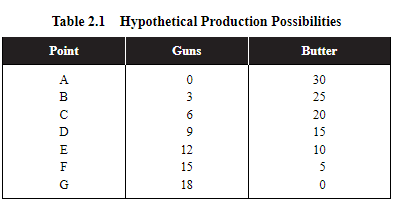
The opportunity cost for guns (D):
(20-15) - (9-6) = (5/3) = 1.67
The opportunity cost for butter (D):
(12-9) - (15-10) = (3/5) = 0.6
\
\
\
Trade-Offs
Since we have scarce resources, individuals, firms, and governments are faced with trade-offs.
- Some examples of trade-offs for individuals are choosing between housing arrangements, transportation options, grocery store items, etc.
- For firms, the trade-offs are often centered on which good or service can be provided, how much should be produced, and how to go about producing those goods and services.
- The government is faced with issues that are likely to have an immediate impact on the lives of local citizens.
</p>
1.2 Opportunity Cost and the Production Possibilities Curve (PPC)
Production Possibilities Curve
- To examine production and opportunity cost, economists find it useful to create a simplified model of an individual, or a nation, that can choose to allocate its scarce resources between the production of two goods or services.
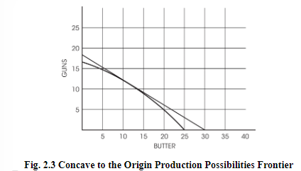
- Realistically, PPC curves are not straight lines and tend to be concave-shaped.
\
\
\
\
The reason for this concave shape is that certain resources are more compatible with the production of a specific good/service.
Thus, when they are used up forcefully, they are less productive-hence the higher opportunity cost arises.
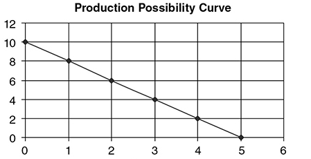
A generalized view of the production possibility curve:
<br /> <br />
<br /> <br /> </p>
- The slope of the curve measures the opportunity cost of the good on the x-axis.
- The inverse of the slope measures the opportunity cost of the good on the y-axis.
</p>
Constant Opportunity Cost v/s Increasing Opportunity Cost
The production possibilities curve can illustrate two types of opportunity costs:
- Increasing opportunity costs:
- We must weigh the benefits and costs of our choices.
- Opportunity cost is the cost of the next best alternative that we must give up pursuing a certain action.
- For instance, if we have $10 and we choose to buy coffee for $2, the opportunity cost is the pastry we could have purchased instead.
- The opportunity cost increases with every decision we make, as we give up more alternatives. This is called increasing opportunity cost.
- It's crucial to consider the opportunity cost of each decision to make the most efficient use of our resources and maximize our benefits.
- Decreasing opportunity costs:
- To decrease opportunity costs, increase efficiency by using fewer resources to achieve the same output.
- Prioritize important goals and allocate resources towards them to minimize the opportunity cost of not pursuing other goals.
- Increase flexibility by adapting quickly to changing circumstances and being open to new ideas.
- The graph for decreasing opportunity curve is not possible in real life.
Efficiency
Productive efficiency - When the economy is producing the maximum output for a given level of technology and resources. All points on the production frontier are productively efficient.
Allocative efficiency - The economy is producing the optimal mix of goods and services.
- Optimal - The combination of goods and services that provides the most net benefit to society.
Market failure - When a market fails to produce the allocative efficient quantity.
</p>
Growth
- Economic growth - The ability to produce a larger total output over time. Can occur if one or all of these happen:
- An increase in the number of resources.
- An increase in the quality of existing resources.
- Technological advancements in production.
- Economic contraction - It is when a country's economy shrinks due to factors such as reduced spending by consumers, businesses, or the government.
- Economic contractions are a normal part of the business cycle and can lead to long-term growth if managed correctly.
\
1.3 Comparative Advantage and Trade
Comparative Advantage and Specialization
Absolute advantage -
- The absolute advantage is producing goods/services more efficiently, using fewer inputs.
- Let’s say a bakery and a pizza parlor both produce pizza crusts and pastries.
<br /> <br />
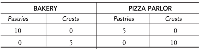
<br /> <br /> This graph presents the number of pastries and crusts each shop can produce. Since the bakery can produce more pastries than the pizza parlor, the bakery has an absolute advantage in pastry production.
Comparative advantage -
- In macroeconomics, this principle is the basis for showing how nations can gain from free trade%%.%% Using the same example as before, we can say that the bakery has a comparative advantage since it can produce pastries at a lower opportunity cost. In the same way, the pizza parlor has a comparative advantage in pizza crusts.
- They describe the way that individuals, nations, and societies can acquire more goods at a lower cost.
There are two types of problems:
- Output problems:
- To determine the absolute advantage, you are simply looking for which country can produce a higher amount of goods or services.
- To determine you have to calculate per unit opportunity cost using the formula give up/gain (the amount of good you are giving up divided by the amount of good you are gaining). Once you have calculated per unit opportunity cost, the country with the lowest one has a comparative advantage.
- If the two countries can both make the same amount of the good, then we say neither country has an absolute advantage.
- Countries export what they have a comparative advantage in and import what they don't have a comparative advantage in.
- Input problems:
- To determine absolute advantage, you are looking for the country that uses the least number of resources (i.e., the lower number).
- To determine comparative advantage, you have to calculate the per unit opportunity cost using the formula gain/give up. Once you have calculated the per unit opportunity cost the country with the lowest one has a comparative advantage.
- If the two countries can both make one unit of the good with the same number of resources, then we say neither country has an absolute advantage.
- Countries export what they have a comparative advantage in and import what they don't have a comparative advantage in.
</p>
Terms of trade:
- It deals with the country’s export prices to income prices and determines the relative price between the nation’s exports and imports.
1.4 Demand
Law of demand - Holding all else equal, when the price of good rises, consumers decrease the quantity demanded of that good.
All else equal - To predict how a change in one variable affects a second, we hold all other variables constant. This is also referred to as the ceteris paribus assumption.
</p>
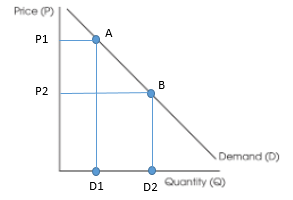
Change in Quantity Demanded vs. Change in Demand
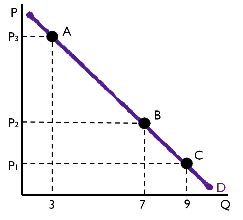
Change in the quantity demanded only occurs due to change in price-movement along the curve.
If product A would become expensive (P2 to P1), the quantity demanded would fall (D2 toD1)
<br />
<br /> </p>
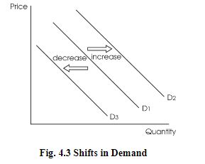
Changes in demand are when the entire curve would shift upwards or downwards.
\
\
\
\
These are the determinants of demand which are variables causing consumers to buy more or less of a product, irrespective of the price.
</p>
Determinants of Demand
- The INSECT Acronym:
- I = Income:
- Goods are usually categorized into 2 types, inferior and normal.
- Demand tends to decline (shift downwards) for inferior goods with an increase in consumer income.
- Demand for normal goods increases (shifts upwards) with an increase in consumer income.
- N = Number of Buyers/Consumers
- The bigger the market for a product, the more likely the demand curve would shift upwards.
- S = Substitutes
- 2 goods would be considered substitutes if an increase in the price of one good cause an increase in demand for the other good.
- E = Expectations of Future Price
- Consumer expectation plays a major role in the determination of the price.
- C = Complements
- These goods are purchased separately but used together.
- T = Tastes and Preferences
- This is the consumer’s taste for a product at any point.
- Summing up:
- Demand increases:
- I = increase
- N = increase
- S = increase
- E = increase
- C = decrease
- T = increase
- Demand decreases:
- I = decrease
- N = decrease
- S = decrease
- E = decrease
- C = increase
- T = decrease
1.5 Supply
Supply is the different quantities of goods and services that are willing to produce at various price levels.
Law of supply -
- Rising prices give greater opportunities for suppliers to earn a profit.
- When the price level increases, the quantity of a good, supplied increases.
- When the price level decreases, the quantity of a good, supplied decreases.
Quantity Supplied v/s Supply
Quantity supplied is the amount of a good or service that is produced at a particular price level.
The quantity supplied is one point on the curve.
Demand is the entire line with all of the points that make it up.
<br />
</p>
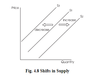
- The change occurs along the supply curve.
<br /> <br />
<br /> </p>
- Shift in supply is due to the determinants of supply.
- Determinants of supply are the factors that influence the supplier to offer more or fewer goods at the same price.
Determinants of Supply
- The ROTTEN Acronym:
- R = Resources
- The cost of production (land, labor, capital) has an inverse impact on the supply.
- When the cost of these increases, the supplier decides to produce less of the products since he is unable to afford the production cost.
- O = Other good prices
- Suppliers who produce more than one product (profit-maximizing firms) have an easier time switching to the production of another product if issues do arise in prices.
- T = Taxes
- Taxes are added up to the unit cost of production, thus making it more expensive.
- T = Technology
- Newer technology causes the cost of production to decline and helps improve the efficiency of the supplier.
- E = Expectations of the supplier
- If suppliers expect prices to increase in the future, they will hold back supply for the current time with the future goal of earning more profit later (and vice versa).
- N = Number of competitors
- As the number of sellers increases in the market, the supply automatically increases.
- This allows consumers more choices at a lower price due to an increase in competition.
- Summing up:
- Supply increases:
- R = increase
- O = decrease
- T = decrease (taxes)
- T = increase (technology)
- E = increase
- N = decrease
- Supply decreases:
- R = decrease
- O = increase
- T = increase (taxes)
- T = decrease (technology)
- E = decrease
- N = increase
1.6 Market Equilibrium
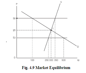
Market Equilibrium
- The market equilibrium price is that price that the market sets, where buyers buy the exact amount which the sellers are willing to produce.
- It’s also known as market-clearing price.
\
\

\
Market Disequilibrium
- This occurs when there is a shortage or surplus in the market.
\
\
\
- Consider the price of $8 where the demand is 100 and the corresponding supply is 350.
- This surplus is what creates market disequilibrium.
Changes in Equilibrium (solving demand and supply-related questions)
- Is it supply, demand, or both?
- Is it an increase (shift to the right) or a decrease (shift to the left)?
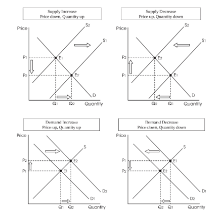
Supply increases towards the right and decreases towards the left.
Demand increases towards the right (moves upwards) and decreases towards the left (moves downwards).
<br /> <br />
<br /> </p>
- When supply is constant and only demand increases, equilibrium price, and quantity increase.
- When supply is constant and only demand decreases, equilibrium price and quantity decrease.
- When demand is constant and only supply increases, equilibrium price, and quantity decrease.
- When demand is constant and only supply decreases, equilibrium price and quantity increase.
Key concepts:
- Market shortage: shortage (Excess demand) - Also known as excess demand, a shortage exists at a market price when the quantity demanded exceeds the quantity supplied. The price rises to eliminate a shortage.
- Market surplus: Surplus (Excess supply) - Also known as excess supply, a surplus exists at a market price when the quantity supplied exceeds the quantity demanded. The price falls to eliminate a surplus.
Changes in equilibrium:
- Increase in demand:
- eq (price) = increases
- eq (quantity) = increases
- Decrease in demand:
- eq (price) = decreases
- eq (quantity) = decreases
- Increase in supply:
- eq (price) = decreases
- eq (quantity) = increases
- Decrease in supply:
- eq (price) = increases
- eq (quantity) = decreases
%%Unit 2: Economic Indicators and the Business Cycle%%
In unit 2, we will dive into all the indicators that economists use to explain the health of the economy.
2.1 Circular Flow and GDP
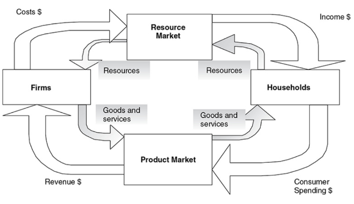
The Circular Flow Model
- Circular flow of economic activity - A model that shows how households and firms circulate resources, goods, and incomes through the economy. This basic model is expanded to include the government and the foreign sector.
- Closed economy - A model that assumes there is no foreign sector (imports and exports).
\
\
\
Now, let’s dive into the components of the circular flow diagram.
Consumers:
- Consumers are the people who buy the goods/services in an economy.
- So, technically everyone is a consumer.
- Consumers send money to the product market by buying goods.
- They also interact with the factor market in which they provide labor and receive wages or income.
Firms:
Producers in the economy.
Firm is any business that produces goods and supplies them to the product market and then receives the payment for those goods.
Firms receive factors of production from the factor market and then pay them with wages.
</p>
Product Market
- The market where firms sell goods and services.
- A sweet exchange of goods and services for money between firms and households.
- Plays a crucial role in the economy.
- The interaction between demand and supply in the product market determines:
- Prices of goods and services
- The number of goods and services that are exchanged.
Factor Market
- The market where factors of production such as labor, capital, and land are bought and sold.
- These factors are used by firms to produce goods and services, which are then sold to households in the goods market.
Gross Domestic Product (GDP)
Gross domestic product (GDP) - The market value of the final goods and services produced within a nation in a given period.
Aggregate spending (GDP) - The sum of all spending from four sectors of the economy. GDP = C + I + G + (X – M).
- Consumer spending (C) - Spending done by customers.
- Investment spending (I) - Investment is defined as current spending to increase output or productivity later.
Three general types of investment are included in GDP:
- New capital machinery purchased by firms.
- New construction for firms or consumers.
- The market value of the change in unsold inventories.
- Government spending (G) - Purchases made by the government for final goods and services and investments in infrastructure.
- Net exports (X– M) - Exports → X, Imports → M
K.I.S.S.: Keep It Simple, Silly
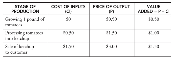
GDP = C + I + G + (X - M) = Aggregate Spending = Aggregate Income (Y) = Sum of all value added
National Income Concepts
Aggregate income (AI) - The sum of all income—Wages + Rent + Interest + Profit—earned by suppliers of resources in the economy. With some accounting adjustments, aggregate spending equals aggregate income and also equals the sum of the value added.
</p>
Value-added approach - A third approach to calculating GDP that considers all stages of production of a final good and the value that was added to the final good along the way.
<br /> <br />
<br /> What is not included in GDP?
Illegal Activities:
- transactions concerning illegal activities like drug trafficking, gambling, etc.
Unpaid work:
- Volunteering and caregiving are not included in GDP.
- not a market transaction.
Transfer payments:
- not represent the production of goods and services.
- like social security benefits or unemployment insurance.
Intermediate goods:
- the goods used in the process but not counted for final consumption.
Depreciation:
- wear and tear on capital goods, such as machines or buildings is not included.
</p>
2.2 Limitations of GDP
Uses of GDP in Economics
1. Measuring Economic Growth
- GDP is used to measure the economic growth of a country. It provides a way to compare the economic performance of different countries over time.
- A higher GDP indicates that the economy is growing, while a lower GDP indicates that the economy is contracting.
2. Comparing Living Standards
- GDP per capita is used to compare the living standards of different countries.
- It measures the average income per person in a country.
- Countries with higher GDP per capita generally have higher living standards.
3. Assessing Business Cycles
- GDP is used to assess the business cycles of a country. Business cycles refer to the fluctuations in economic activity over time.
- GDP can be used to identify periods of economic expansion and contraction.
4. Formulating Economic Policies
- GDP is used to formulate economic policies. Governments use GDP data to make decisions about fiscal and monetary policies.
- For example, if GDP is growing too slowly, the government may implement policies to stimulate economic growth.
5. Attracting Foreign Investment
GDP is used to attract foreign investment.
Countries with higher GDPs are generally seen as more attractive to foreign investors.
This is because a higher GDP indicates a more stable and prosperous economy.
</p>
Limitations of GDP
There are 4 main areas of limitation of GDP:
Acronym: P-I-E-S
1. Population
- When populations are different from country to country but produce a similar amount of products.
- This gives an inaccurate picture of GDP.
2. Inequality
- It’s a limit in measuring the standard of living.
- Two countries with the same GDP but unequal distribution of income among all.
3. Environment
- It’s a limit to measure the health of the economy.
4. Shadow economy
- It involves the items which are not counted in GDP.
- Shadow economy is the black market.
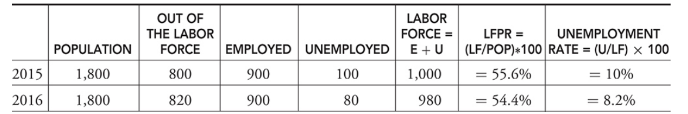
2.3 Unemployment
- Employed - A person is employed if they have worked for pay at least one hour per week.
- Unemployed - A person is unemployed if they are not currently working but are actively seeking work.
Measuring the Unemployment Rate
- Labor force - The sum of all individuals 16 years and older who are either currently employed (E) or unemployed (U). LF = E + U.
- Out of the labor force - A person is classified as out of the labor force if they have chosen to not seek employment.
- Labor force participation - The ratio of the size of the labor force to the size of the population 16 years and older. LFPR = (LF/Pop)*100.
- Unemployment rate - The percentage of the labor force that falls into the unemployed category. Sometimes called the jobless rate. UR = 100 × U/LF.
\
\
\
\
- Discouraged workers - Citizens who have been without work for so long that they become tired of looking for work and drop out of the labor force. Because these citizens are not counted in the ranks of the unemployed, the reported unemployment rate is understated.
Types of Unemployment
- Frictional unemployment - A type of unemployment that occurs when someone new enters the labor market or switches jobs. This is a relatively harmless form of unemployment and is not expected to last long.
- Seasonal unemployment - A type of unemployment that is periodic, predictable, and follows the calendar. Workers and employers alike anticipate these changes in employment and plan accordingly, thus the damage is minimal.
- Structural unemployment - A type of unemployment that is the result of fundamental, underlying changes in the economy such that some job skills are no longer in demand.
- Cyclical unemployment - A type of unemployment that rises and falls within the business cycle. This form of unemployment is felt economy-wide, which makes it the focus of macroeconomic policy.
Full Employment
- Full employment - Exists when the economy is experiencing no cyclical unemployment.
- The natural rate of unemployment - The unemployment rate associated with full employment, somewhere between 4 to 6 percent in the United States.
2.4 Prices Indices and Inflation
The Consumer Price Index (CPI)
Consumer price index (CPI) - The price index that measures the average price level of the items in the base year market basket. This is the main measure of consumer inflation.
Deflation: the general decrease in prices.
Inflation: the general increase in prices.
Disinflation: a decrease in the rate of inflation.
Inflation rate: the percentage change in aggregate price level across an entire economy in a year.
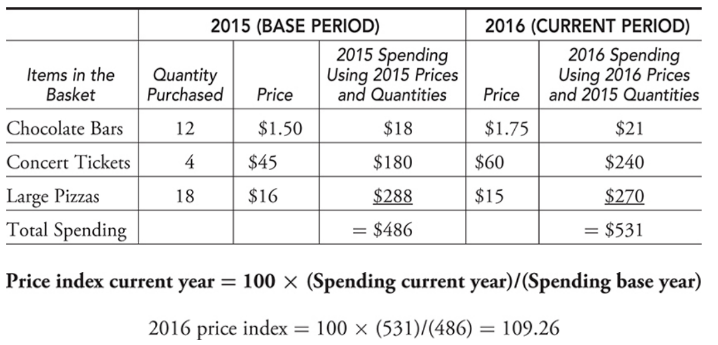
Market basket - A collection of goods and services used to represent what is consumed in the economy.
<br /> <br />
<br /> </p>
Inflation
- Inflation - The percentage change in the CPI from one period to the next.
- The annual rate of inflation on goods consumed by the typical consumer - The percentage change in the CPI from one year to the next.
- Ex. → In January 2000, the CPI was 169.30, and one year later in January 2001, it had risen to 175.60. We need to calculate the percentage change in the CPI to calculate inflation. Inflation = (175.60 — 169.30)/169.30 = .037 or 3.7%
Difference between CPI and GDP Deflator
- The CPI is based on a market basket of goods bought by consumers, including the ones produced abroad. It’s a measure of inflation of only consumer goods.
- Consumer Inflation rate = 100 x (CPI new - CPI old)/ CPI old
- The GDP deflator includes all items that make up domestic products. It includes more than just consumer goods, so it’s a broader measure of inflation.
Nominal and Real Income
- Nominal income - Today’s income is measured in today’s dollars. These are dollars unadjusted by inflation.
- Real income - Today’s income is measured in base year dollars. These inflation-adjusted dollars can be compared from year to year to determine whether purchasing power has increased or decreased.
- Real income this year = (Nominal income this year)/CPI this year (in hundredths)
- Ex. →In 2014 Kelsey’s nominal income was $40,000, and it increases to $41,000 in 2015. Curious about her purchasing power, she looks up the CPI in 2014 and finds that at the end of that year, it was 234.8; at the end of 2015, it was 236.5. This is compared to the base year value of 100 in 1984.
- Real income 2015 = $40,000/2.348 = $17,036
- Real income 2016 = $41,000/2.365 = $17,336
Difficulties with CPI
- Consumer substitute - As the price of goods begins to rise, we know that consumers seek substitutes. This substitution might make the base year market basket a poor representation of the current consumption pattern.
- Goods evolve - The emergence of new products (smartphones) and the extinction of others (manual typewriters) is understood by firms and consumers, but the market basket must reflect this or it risks becoming irrelevant.
- Quality differences - Some price increases are the result of improvements in quality. Prices that increase because the product is fundamentally better are not an indication of overall inflation. Since the BLS can’t tell the difference between quality improvements and actual inflation, the CPI can be overstated.
2.5 Costs of Inflation
Expected Inflation
- When inflation is predictable, people can plan accordingly. The bank adds an inflation factor on the real rate of interest to create a nominal rate of interest that savers receive and borrowers pay.
- Nominal interest rate = Real interest rate + Expected inflation
- The real rate of interest - The percentage increase in purchasing power that a borrower pays a lender.
Unexpected inflation
- Some people gain and others lose since there’s no time to plan.
- Rapid unexpected inflation usually hurts employees if real wages are falling, as well as fixed-income recipients, savers, and lenders.
- Rapid unexpected inflation usually helps firms if real wages are falling, as well as borrowers. It might also increase the value of some assets like real estate or other properties.
Costs of Inflation
- Menu costs:
- It results from firms having to change prices.
- As inflation occurs, the price just skyrocketed and is placed in like a menu as a result.
- Shoe-leather costs:
- It refers to the time and effort that people end up spending to counterattack the effects of inflation.
- Loss of purchasing power:
- It occurs because inflation causes the value of the individual dollar to decrease over time.
- Wealth distribution:
- It involves the real value of wealth being transferred from one group to another.
2.6 Real v/s Nominal GDP
Real and Nominal GDP
- Nominal GDP - The value of current production at the current prices. Valuing 2015 production with 2015 prices creates nominal GDP in 2015. Also known as current-dollar GDP or money GDP.
- Real GDP - The value of current production but using prices from a fixed point in time. Valuing 2015 production at 2014 prices creates real GDP in 2015 and allows us to compare it back to 2014. Also known as constant-dollar or real GDP.
\
- To deflate the nominal GDP or adjust it for inflation, this division should be made:
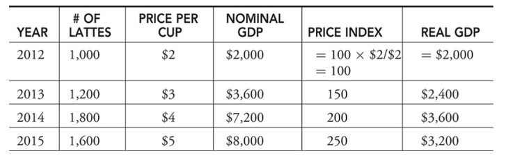
- Real GDP = 100 X (Nominal GDP)/(Price index)
- Real GDP = (Nominal GDP)/(Price index; in hundreds)
- Base year - The year that serves as a reference point for constructing a price index and comparing real values over time
- Price index - A measure of the average level of prices in a market basket for a given year, when compared to the prices in a reference (or base) year. You can interpret the price index as the current price level as a percentage of the level in the base year.
- Latte price index (LPI) example → Suppose GDP is made up of just one product, cups of latte. We need a price index to calculate real GDP. Using 2012 as the base year, a latte index is created and used to adjust nominal GDP to real GDP for this good.
- LPI in year t = 100 x (Price of latte in year t)/ (Price of a latte in base year)
\
\
\
\
Using Percentages
- % ∆ real GDP = % ∆ nominal GDP - % ∆ price index
- If nominal GDP increased by 5 percent and the price index increased by 1 percent, we could say that real GDP increased by approximately 4 percent.
The GDP Deflator
GDP price deflator - The price index that measures the average price level of the goods and services that make up GDP.
</p>
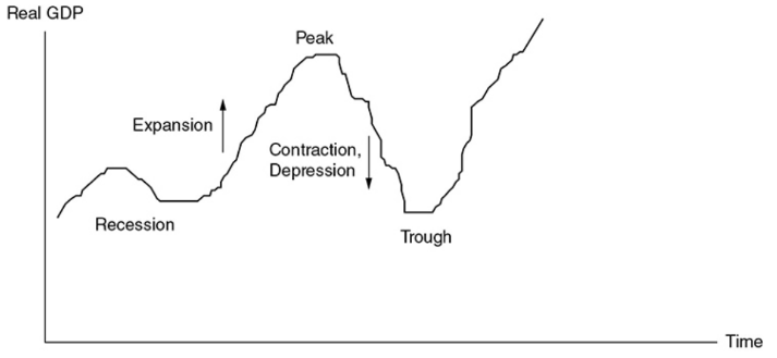
2.7 Business Cycles
The business cycle - The periodic rise and fall in 4 phases present in economic activity. Can be measured by changes in real GDP.
<br /> <br />
<br /> </p>
Expansion - A period where real GDP is growing.
Peak - The top of a business cycle where an expansion has ended.
Contraction - A period where real GDP is falling.
- Recession - Unofficially defined as two consecutive quarters of falling real GDP.
- Depression - A prolonged, deep contraction in the business cycle.
Trough - The bottom of the cycle where a contraction has stopped.
%%Unit 3: National Income and Price Determination%%
3.1 Aggregate Demand
- Aggregate demand (AD) - The inverse relationship between all spending on domestic output and the aggregate price level of that output.
Components of AD
- Demand in the macroeconomy comes from four general sources, which are used to calculate the real GDP.
- AD measures the sum of consumption spending by households, investment spending by firms, government purchases of goods and services, and net exports (exports minus imports).
The shape of AD
General groups of substitutes for national output
- Foreign sector substitution effect - Goods and services produced in other nations.
- Ex. →When the price of U.S. output increases, consumers begin to look for similar items produced elsewhere. A Japanese computer, a German car, and a Mexican textile all begin to look more attractive when inflation heats up in the United States. The resulting increase in imports pushes real GDP down at a higher price level.
- Interest rate effect - Goods and services in the future.
- Ex.→ When more and more households seek loans, the real interest rate begins to rise, and this increases the cost of borrowing. Firms postpone their investment in plant and equipment, and households postpone their consumption of more expensive items for a future when their spending might go further and borrowing might be more affordable. This wait-and-see mentality reduces the current consumption of domestic production as the price level rises and real GDP falls.
- Wealth effect - Money and financial assets.
- Wealth is the value of accumulated assets like stocks, bonds, savings, and cash on hand.
- As the aggregate price level rises, the purchasing power of wealth and savings begins to fall. Higher prices, therefore, tend to reduce the quantity of domestic output purchased.
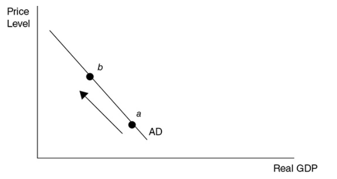
The AD Curve
- The combination of the foreign sector substitution, interest rate, and wealth effects predicts a downward-sloping AD curve.
- As the aggregate price level rises, consumption of domestic output (real GDP) falls along the AD curve. (This is the movement from a to b).
\
\
\
\
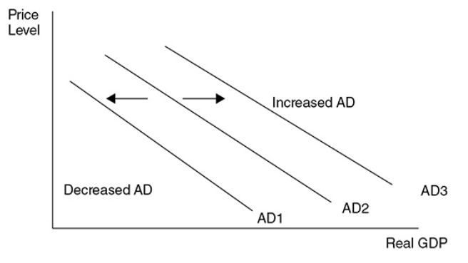
Changes in AD
Since AD is the sum of the four components of domestic spending [C, I, G, (X — M)], if any of these components increases, holding the price level constant, AD increases, which increases real GDP. This is seen as a shift to the right of AD.
If any of these components decreases, holding the price level constant, AD decreases, which decreases real GDP. This is seen as a shift to the left of AD.
<br /> <br />
<br /> </p>
If you want to stimulate real GDP and lower unemployment, you need to boost any or all of the components of AD.
If you feel AD must slow down, you need to rein in the components of AD.
Components of AD
- Consumer Spending (C) - If you put more money in the pockets of households, it is expected that they consume a great deal of it and save the rest. Consumers also increase their consumption if they are optimistic about the future.
- Investment Spending (I) - Firms increase investment if they believe the investment will be profitable. This expected return on the investment is increased if investors are optimistic about future profitability or if the necessary borrowing can be done at a low rate of interest.
- Government Spending (G) - The government injects money into the economy by spending more on goods and services, by reducing taxes, or by increasing transfer payments.
- Government spending on goods and services is a direct increase in AD.
- Lowering taxes and increasing transfer payments increase AD through consumer spending by increasing disposable income.
- Net Exports ( X - M) - When sales to foreign consumers are high and purchases from foreign producers are low, the net exports increase.
- Foreign incomes - Exports increase with strong foreign economies. When foreign consumers have more disposable income, this increases the AD in the United States because those consumers spend some of that income on U.S.-made goods.
- Consumer tastes - If American blue jeans become more popular in France, American AD increases. If French wines become more preferred by American consumers, AD in France increases.
- Exchange rates - Imports decrease when the exchange rate between the dollar and foreign currency falls. This makes foreign goods to be more expensive causing consumers to buy fewer foreign-produced items.
3.2 Spending and Tax Multipliers
Multipliers
- Multiplier effect—The idea that an initial change in spending will set off a spending chain that is magnified in the economy.
- Marginal propensity to consume (MPC)—How much people consume rather than save when there is a change in income. This can also be explained as the portion of each new dollar of disposable income that consumers will spend rather than save.
- Marginal propensity to save (MPS)—How much people save rather than consume when there is a change in income. This can also be explained as the portion of each new dollar of disposable income that consumers will save rather than spend.
MPC and MPS
- Marginal Propensity to Consume (MPC) is calculated by dividing the change in consumption by dividing the change in disposable income.
- Marginal Propensity to Save (MPS) is calculated by dividing the change in savings by dividing the change in disposable income.
- MPC + MPS = 1
Spending Multiplier
- The spending multiplier, or fiscal multiplier, is an economic measure of the effect that a change in government spending and investment has on the Gross Domestic Product of a country. In other words, it measures how GDP increases or decreases when the government increases or decreases spending in the economy.
- Example: Matthew is an economist in the Federal Reserve, and he has been tasked with figuring out the ideal stimulus would be to increase GDP by $5,000,000. He reasons that in order to do that, he needs to figure out how much of their income consumers spend, and how much they save. Through looking at the market and statistical data, he sees that consumers are saving 35% of their after-tax income while spending 65% of it.
- Using the spending multiplier formula (1 / MPS), he calculates that the Federal Reserve needs to inject (5,000,000 / 2.86) = $1,748,251.75 into the economy based on the current MPS.
- Why does the government only have to spend $1.7M to increase GDP by $5M? This is because of the multiplier effect. One group of consumers consumes 65% of its new money on goods produced by another consumer. This consumer now has new money and consumes 65% of it on goods produced by someone else and so on.
- Thus, consumers immediately consume 65 percent of this increase ($1.7M x .65). This $1.1M of consumption then triggers another line of consumption where these consumers consumer 65% of their earnings ( .65 x .65 x $1.7M). This goes on and on resulting in a multiple of 2.86.
- The Spending Multiplier is largely related to how much consumers save, so if they save only 20% of their income and spend the rest, then whatever stimulus the Fed provides is magnified by 5 (1 / (0.2) = 5). This is the reason governments encourage spending during recessions. It can stimulate the economy and increase the flow of money.
Tax Multiplier
The tax multiplier is used to determine the maximum change in spending when the government either increases or decreases taxes.
The tax multiplier is basically the opposite of spending multipliers. It talks about how much people will not spend if taxes increase. If our net worth decreases because of taxes, it's natural for people to cut back on spending right?
- The formula for this multiplier is -MPC/MPS. The tax multiplier will always be less than the spending multiplier. When spending occurs, we know that all of this money will be multiplied in the economy. But, when taxes are increased or decreased, not all the money received goes back into the economy. For example, if the government decreases taxes which gives individuals more disposable income, there is no guarantee they are going to spend all of the additional income.
- Let's look at how we calculate this. If the MPC is 0.8 and the government imposes a $50 increase in taxes, what is the tax multiplier and what happened to the GDP?
tax multiplier = -MPC/MPS
tax multiplier = -0.8/0.2
tax multiplier = -4
GDP change: -4 * $50 = -$200
One fun thing about tax multipliers is the fact that tax multipliers are smaller than spending multipliers. This is because spending multipliers have an immediate impact on the economy, but tax multipliers first have to go through someone's income before having an impact on the economy.
3.3 Short-Run Aggregate Supply (SRAS)
Aggregate supply (AS)
- The relationship between the aggregated price level of all domestic output and the level of domestic output produced.
Short-Run Aggregate supply (SRAS)
- The positive relationship between the level of domestic output produced and the aggregate price level of that output.
Macroeconomic Short Run
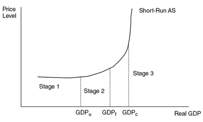
In the macroeconomic short-run period, the prices of goods and services are changing in their respective markets, but input prices have not been adjusted to those product market changes. In the short run, the SRAS curve is typically drawn as upward sloping.
<br /> <br />
<br /> </p>
In stage 1, the economy is in a recession with low production meaning they are many unemployed resources.
In stage 2, real GDP increases and approaches full employment, available resources are harder to find and input costs begin to rise. If the price level for output rises faster than the rising costs, producers have a profit incentive to increase production.
In stage 3, the AS curve is almost vertical, meaning that the economy is growing and approaching the nation’s productive capacity where firms cannot find unemployed units.
- GDPu - Low production
- GDPf - Full employment
- GDPc - Nation’s productive capacity
Changes in AS
- In the short run, AS fluctuates without affecting the level of full employment.
Short-Run Shifts
- The most common factor that affects short-run AS → An economy-wide change in input (or factor) prices.
- Input prices - If input prices fall economy-wide, the short-run AS curve increases without changing the level of full employment.
- Tax policy - Some taxes are aimed at producers rather than consumers. If these “supply-side taxes” are lowered, short-run AS shifts to the right.
- Deregulation - When the regulation of industries restricts their ability to produce, the short-run AS likely increases.
- Political or environmental phenomena - For a nation as large as the United States, wars and natural disasters can decrease the short-run AS without permanently decreasing the level of full employment. For a smaller nation or a large nation hit by an epic disaster, this could be a permanent decrease in the ability to produce.
3.4 Long-Run Aggregate Supply (LRAS)
Long-Run Aggregate supply (LRAS)
- It is defined as the number of goods and services that an economy is capable of producing with the full employment of resources.
Macroeconomic Long Run
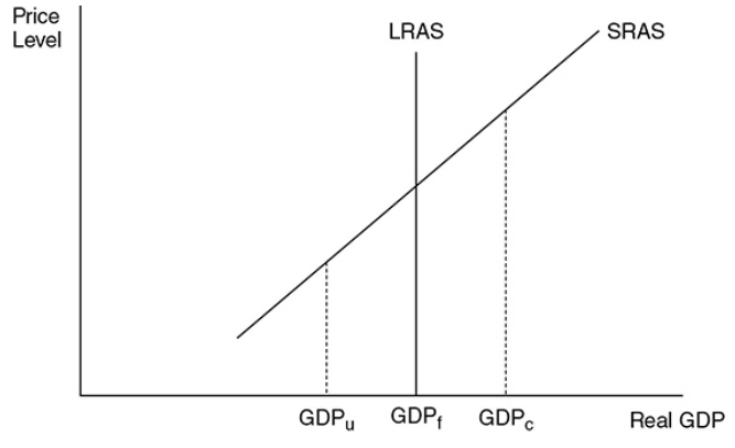
In the macroeconomic long run, the input prices have enough time to fully adjust to market forces. Here all product and input markets are balanced, and the economy is at full employment (GDPf).
The Classical school of economics asserts that the economy always gravitates toward full employment, so a cornerstone of classical macroeconomics is a vertical AS curve.
<br /> <br />
</p>
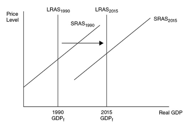
Long-Run Shifts
Availability of resources - A larger labor force, a larger stock of capital, or more widely available natural resources can increase the level of full employment.
Technology and productivity - Better technology raises the productivity of both capital and labor. A more highly trained or educated populace increases the productivity of the labor force.
Policy incentives - If the policy provides large incentives to quickly find a job, full-employment real GDP rises. If the government gives tax incentives to invest in capital or technology, GDPf rises.
- Ex. → Since the 1990s, the U.S. economy has seen dramatic increases in technology and investment in capital stock. This period produced a significant increase in the real GDP at full employment.
<br /> <br />
<br /> </p>
When the LRAS curve shifts to the right, it indicates economic growth.
3.5 Equilibrium in Aggregate Demand-Aggregate Supply (AD-AS) Model
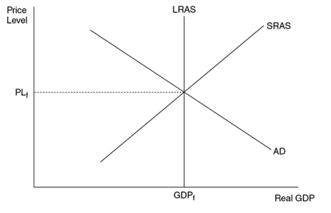
Equilibrium Real GDP and Price Level
Macroeconomic equilibrium - Occurs when the quantity of real output demanded is equal to the quantity of real output supplied. Graphically this is at the intersection of AD and SRAS. Equilibrium can exist at, above, or below full employment.
<br /> <br />
<br /> </p>
\
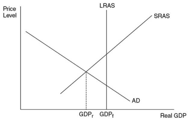
Recessionary and Inflationary Gaps
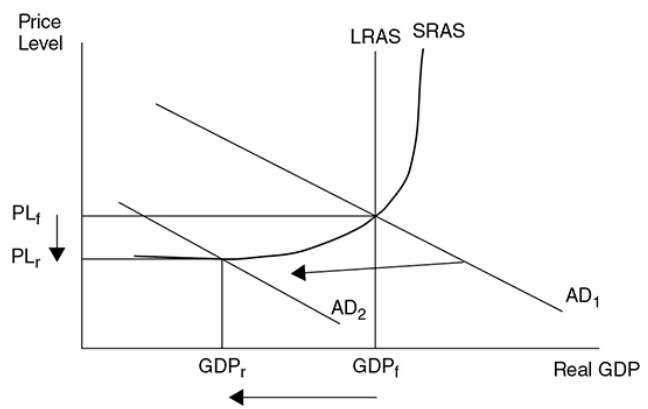
Recessionary gap - The amount by which full-employment GDP exceeds equilibrium GDP.
<br /> <br />
<br /> </p>
In this picture, the recessionary gap is the difference between GDPf and GDPr, or the amount that the current real GDP must rise to reach GDPf.
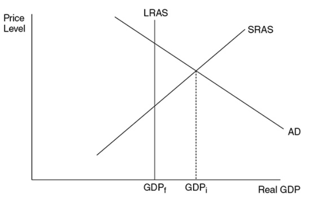
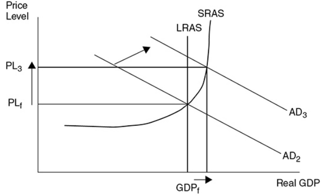
Inflationary gap - The amount by which equilibrium GDP exceeds full employment GDP.
<br /> <br />
<br /> </p>
In this picture, the inflationary gap is the difference between GDPi and GDPf, or the amount that real GDP must fall to reach GDPf.
3.6 Changes in the AD-AS Model in the Short Run
GDP Determinants
- Consumer spending
- Investment spending
- Government spending
- Net exports (exports-imports)
Supply Shocks
Supply shocks - An economy-wide phenomenon that affects the costs of firms and the position of the SRAS curve, either positively or negatively. The shifts in SRAS are caused by these.
<br /> <br />
<br /> </p>
Positive supply shocks might be the result of higher productivity or lower energy prices.
Negative supply shocks usually occur when economy-wide input prices suddenly increase. ^^Ex. →^^ The Gulf War of 1990 to 1991.
3.7 Long-Run Self-Adjustment
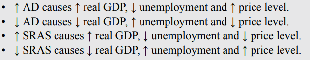
Adjustment to a Recessionary Gap
\
\
\
- Based on this graph, the economy is currently operating at full employment. If consumers and firms begin to lose confidence in the labor market and overall economy, AD shifts to the left.
- In the short run, this causes a recessionary gap as real GDP falls to GDPr meaning that unemployment rises and aggregate price levels fall from PL1 to PL2.
- NOTE - One of the hallmarks of a recession is a decreased demand for many factors of production.
- This recessionary gap fixes itself since the prices of the products will decrease, causing a gradual rightward shift of the SRAS curve to SRAS2. The curve shifts to the right until the gap is closed and the economy is back at GDPf.
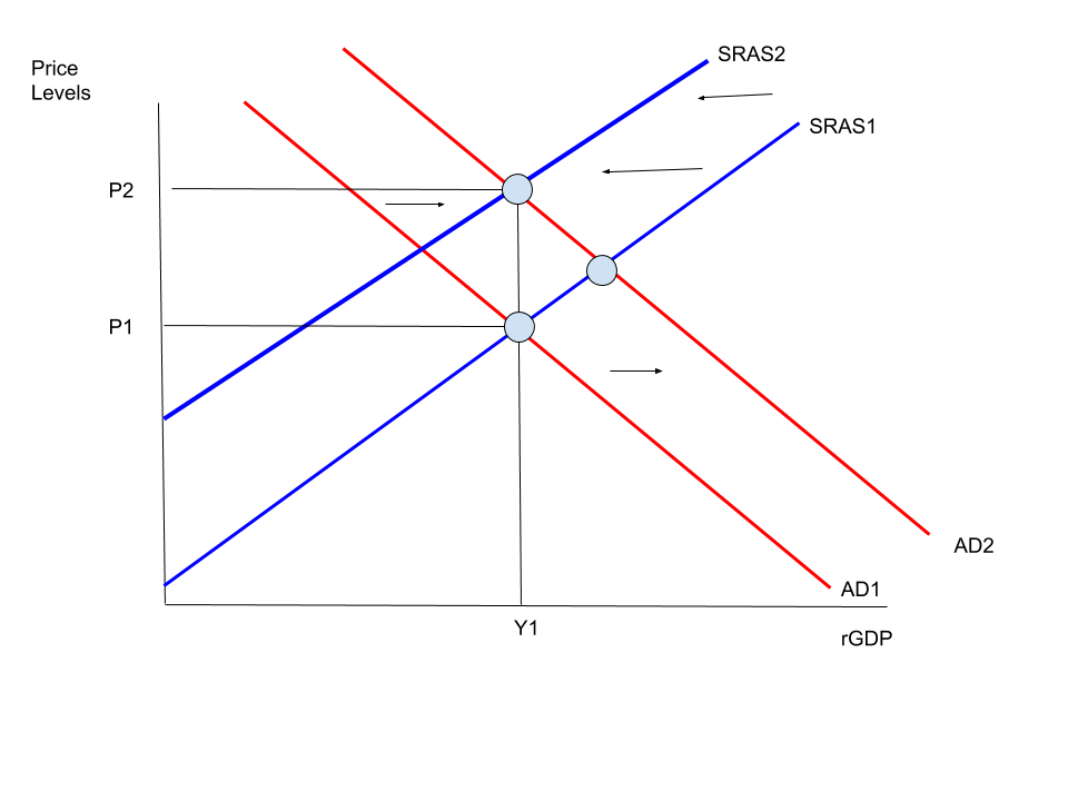
Adjustment to an Inflationary Gap
\
\
\
- When the AD curve increases, an inflationary gap happens to cause an increase in real GDP to GDPi (lower unemployment rate) and an increase in the aggregate price level to PL2.
- When this happens, there’s stronger demand for labor and all of the other factors of production causing factor prices to rise. As the factor prices rise, the SRAS curve shifts to the left to SRAS2 eventually eliminating the inflationary gap, but at a higher aggregate price level of PL3.
3.8 Fiscal Policy
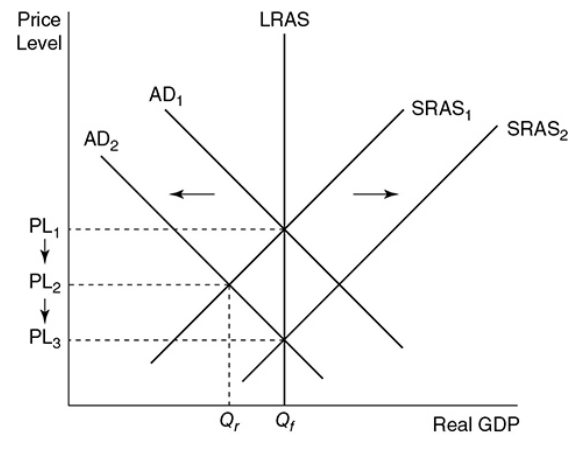
Expansionary Fiscal Policy
Fiscal policy - Deliberate changes in government spending and net tax collection affect economic output, unemployment, and the price level. Fiscal policy is typically designed to manipulate AD to “fix” the economy.
Expansionary fiscal policy - Real GDP is low and unemploymentis high when the economy suffers a recession. In the AD and AS model, there’s a recessionary equilibrium located below full ememployment
<br /> <br />
<br /> </p>
If the government increases the spending or lowers net taxes, the AD curve increases. If taxes are lowered, the multiplier is smaller so to have the same increase in real GDP, the amount of taxes cut has to be larger than an increase in government spending.
To resume, expansionary fiscal policy is the increases in government spending or lower net taxes meant to shift AD to the right.
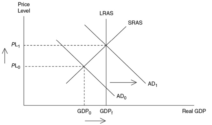
Contractionary Fiscal Policy
Contractionary fiscal policy - When the economy operates beyond full employment, inflation becomes a problem, so the government might need to contract the economy. This inflationary equilibrium is beyond full employment. It can be done by decreasing government spending or increasing net taxes, opposite to expansionary fiscal policy. Both of these options causes the AD to shift to the left with the purpose of decreasing real GDP and decreasing inflation.
<br /> <br />
<br /> </p>
To resume, contractionary fiscal policy decreases government spending or increases net taxes to shift AD to the left.
Sticky prices - If price levels do not change, especially downward, with changes in AD, then prices are thought of as sticky or inflexible. Keynesians believe the price level does not usually fall with contractionary policy.
- On the other hand, Classical school economists believe that the long-run economy adjusts naturally to full employments they see the AS curve as vertical. This implies that prices are flexible and can rise and fall, as seen in the last graph.
Short-Run Effects
- Lags and delays can sometimes occur with the discretionary fiscal policy.
- Non-discretionary fiscal policy refers to permanent spending or taxation laws already on books that help regulate the economy.
Calculating Fiscal Policies
For government to help this economy correct itself back to the long-run:
- to decide the amount of adjustment in taxes
- goal: to shift aggregate demand to right in doing it back to where it connects SRAS AND LRAS at same GDP level.
If we said that the MPC was .5, then that means that the MPS is also .5. If you remember from section 3.2, MPC + MPS always equals 1. The spending multiplier is calculated by dividing 1/MPS. So in this particular situation, the spending multiplier would be 2. This means that for every dollar the government spends, it will multiply twice in the economy. Since there is a gap of $50 billion than the governmthencould correct this economy by spending $25 billion.
Since the MPC is .5, we would calculate the tax multiplier as .5/.5 (MPC/MPS). This would make the tax multiplier 1. So in order to correct this particular economy, the government would have to decreases taxes by $50 billion (the entire value of the gap).
3.9 Automatic Stabilizers
Automatic Stabilizers
- A type of fiscal policy that is already in place to offset the fluctuations or economic activity in our economy.
- It is typically used to counter the effects of negative supply shocks or recessions.
- Do not prevent anything.
- Income taxes and anti-poverty programs are examples of automatic stabilizers during an economic boom or recession.
Recessionary Period
- During a recession, less people are employed and less income is made for those unemployed families.
- If people have less money, they will spend less, worsening the economy.
- Programs like TANF (Temporary aid to needy families) will come to rescue.
- When more people are unemployed, more people will qualify for TANF, and more people will receive money from the government. This will, in turn, increase temporary "income" for the unemployed families, and they'll likely spend more. This will help the economy regain its strength with the help of increased spending.
- When the economy is improved, fewer families will qualify for TANF, which will lead to the size of the program decreasing. Less families will receive aid through TANF, so that the government is not always spending money.
Inflationary Period
- When inflation is rapidly increasing, income taxes will kick into effect. During the economic boom, the problem is that too many people are spending way too much.
- The government's income taxes can soothe this boom a little.
- Progressive income taxes describe income taxes that tax more if that household earns more income.
%%Unit 4: Financial Factor%%
4.1 Financial Assets
Financial Assets
- The firm invests in a physical asset if the expected rate of return is at least as high as the real interest rate.
- Financial investments yield a rate of return.
Key Terms:
- Liquidity:
- The ease with which a financial asset can be assessed and converted into cash.
- Most liquid asset: Cash
- Rate of return:
- Net gain/loss of an investment over a specified period.
- Preference is given to investments with a higher rate of return.
- Risk:
- The chance that an outcome or an investment’s actual gains differ from the expected outcome.
Stocks
- Stock - A certificate that represents a claim to, or share of the ownership of a firm.
- Equity financing - The firm’s method of raising funds for investment by issuing shares of stock to the public.
Bonds
- Bond - A certificate of indebtedness from the issuer to the bondholder.
- When a firm wants to raise money by taking a loan (borrowing money), it can issue corporate bonds that promise the bondholders the principle amount plus interest with repayment on a specific date. This is a form of debt financing.
- Bonds can be bought and sold in a secondary market.
- Debt financing - A firm’s way of raising investment funds by issuing bonds to the public.
Loans
- The process of borrowing money and repaying it with interest.
- example: credit cards
Bank Deposits
- The money in your bank account.
- Checking account or Demand deposits.
- Money can be used whenever you want.
- No interest.
- example: debit cards
Bonds and Interest Rates
- Bond prices and interest rates have an inverse relationship.
- People prefer higher interest rates as they are given a greater rate of return.
- Bonds pay fixed interest rates, as interest rates fall, the price rises.
- If interest rates are on a rise, consumers are less interested in fixed interest rates of bonds, and the price falls.
4.2 Nominal v/s Real Interest Rates
Interest Rates
It includes two types of interest rates:
- Nominal interest rate
- Real interest rate
Equation:
Nominal interest rate = real interest rate + inflation
Real interest rate = nominal interest rate - inflation
| Nominal Interest Rates | Real Interest Rates |
|---|---|
| Not adjusted for inflation | Adjusted for inflation |
| Measures the price of money and reflects current rates and market conditions | Measures purchasing power and shows how much you or a lender actually earned from interest paid |
Predictions
- When nominal interest rates are higher than inflation rates, real interest rates are positive.
- When nominal interest rates are lower than inflation rates, real interest rates are negative.
- Nominal and real interest rates are important because they play different roles in your financial decisions.
- If a real interest rate is positive, it means you have more purchasing power.
- If the real interest rate is negative, then it means you have less purchasing power—at least when it comes to investments and earning interest on your money.
- When it comes to borrowing money, negative real interest rates may influence borrowers, such as potential homeowners who see low-interest rates as an attractive time to buy, thus pushing up the demand for houses and their prices.
- At the same time, businesses may be more inclined to borrow money to finance projects or acquisitions. On the other hand, conservative investors may face difficult choices as to where to put their money.
4.3 Definition, Measurement, and Functions of Money
Types of Money
- Fiat Money: The paper and coin money used today. Since it has no intrinsic value, it is backed by the public’s trust that the government maintains its value.
- Commodity Money: It is something that performs the function of money and has an alternative, non-monetary use.
- examples: tobacco, silver, gold, oil, precious metals, etc.
Functions of Money
- Functions of money - Money serves three functions. It serves as a medium of exchange, a unit of account, and a store of value.
- Medium of exchange - It follows the logic that your labor hours turn into money, the money turns into apples, the farmer then exchanges the money for an orchard’s apple crop, and so on.
- Unit of account - Units of currency measure the relative worth of goods and services. In a barter economy, the value of a pound of cheese would equal a dozen eggs. With money, the value of goods is measured in a monetary unit.
- Store of value - Money is a relatively good way to store value, when there’s no inflation because it keeps its value. A cheese maker would have to sell the cheese before it gets moldy to earn a profit.
Supply of Money
- Money supply - The quantity of money in circulation as measured by the Federal Reserve (the Fed) as M1 and M2. It is assumed to be fixed at a given point in time.
- Liquidity - A measure of how easily an asset can be converted to cash. The more easily it can be converted to cash, the more liquid the asset is.
- M1 - The most liquid of money definitions and the basis for all other more broadly defined measures of money. M1 = Cash + Coins + Checking deposits + Traveler’s checks.
- M2 - It is less liquid than M1. M2 = M1 + Savings deposits + Small time deposits + Money market deposits + Money market mutual funds.
- At any point in time, the supply of money is constant, meaning that the current money supply curve is vertical.
Monetary Base (MO/MB)
- Money circulation or in the bank reserves.
- Physical paper and coin currency used by the economy.
- Not included in the money supply.
- Details the final settlement for the transaction.
- example: if you use cash to pay off the debt it’s a monetary base whereas using a credit card would not be a monetary base.
- Monetary base = currency in circulation + bank reserves
4.4 Banking and the Expansion of the Money Supply
Fractional Reserve Banking
- Fractional reserve banking - A system in which only a fraction of the total money deposited in banks is held in reserve as currency.
- Reserve ratio (rr) - The fraction of a bank’s total deposits that are kept on reserve.
Money Creation
- Reserve ratio (rr) = Cash reserves/Total deposits.
- Reserve requirement - Regulation set by the Fed that states the minimum reserve ratio for banks.
- Excess reserves - The cash reserves held by banks above and beyond the minimum reserve requirement.
- T-account or balance sheet - A tabular way to show the assets and liabilities of a bank. Total assets must equal liabilities.
- Asset of a bank - Anything owned by the bank or owed to the bank is an asset of the bank.
- Reserve cash is an asset and so are loans made to citizens.
- Liability of a bank - Anything owned by depositors or lenders is a liability to the bank.
- Checking deposits of citizens or loans made to the bank are liabilities to the bank.
- Ex. → Katie takes $1,000 from under her mattress, deposits it at ECB, and opens a checking account. If the Federal Reserve tells the ECB that it must hold 10 percent of all deposits in reserve, then the ECB must comply and keep no less than $100 of Katie’s deposit as “required” reserves. The remaining $900 of the deposit are excess reserves and can be kept on reserve in the bank or lent to another person.
The Money Multiplier
- Money multiplier - This measures the maximum amount of new checking deposits that can be created by a single dollar of excess reserves. M = 1/(reserve ratio) = 1/rr. The money multiplier is smaller if:
- At any stage the banks keep more than the required dollars in reserve
- At any stage borrowers do not redeposit funds into the bank and keep some as cash
- Customers are not willing to borrow.
- An initial amount of excess reserves multiplies by a factor of M, at most.
4.5 The Money Market
Demand for Money
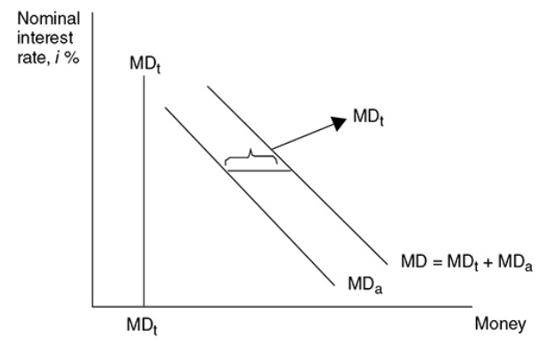
Transaction demand - The amount of money held in order to transactions. This is not related to the interest rate, but it increases as nominal GDP increases.
Ex. → If nominal GDP is $1,000 and each dollar is spent an average of four times each year, money demand for transactions would be $1,000/4 = $250. If nominal GDP increases to $1,200, money demand for transactions increases to $1,200/4 = $300.
Asset demand - The amount of money demanded as an asset. As nominal interest rates rise, the opportunity cost of holding money begins to rise and you are more likely to lessen your asset demand for money.
Total demand - Plotted against the nominal interest rate, the transaction demand for money is a constant MDt. Adding this constant needed to make transactions to a downward-sloping asset demand for money (MDa) creates the total money demand curve.
<br /> <br />
<br /> </p>
- Money demand - The demand for money is the sum of money demanded transactions and money demanded as an asset. It is inversely related to the nominal interest rate.
Shifters of the Demand for Money Curve
- Price Level
- Real GDP
- Transaction Costs
The Supply of Money
- The monetary base of a nation is determined by the country’s central bank (FED).
- Money supply is independent of the nominal interest rate.
- The Federal Reserve has three general tools of monetary policy that they control:
- Engaging in open market operations
- Changing the discount rate
- Changing the required reserve ratio
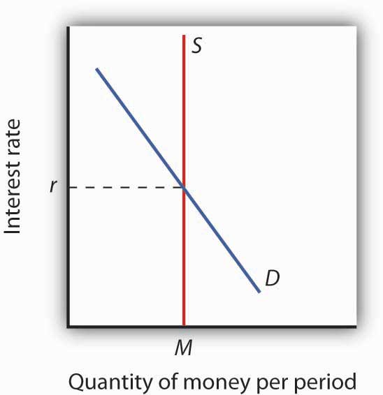
Money Market Equilibrium
- The money market is the interaction among institutions through which money is supplied to individuals, firms, and other institutions that demand money.
- Money market equilibrium occurs at the interest rate at which the quantity of money demanded is equal to the quantity of money supplied.
\
\
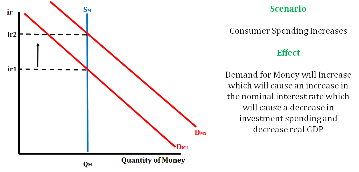
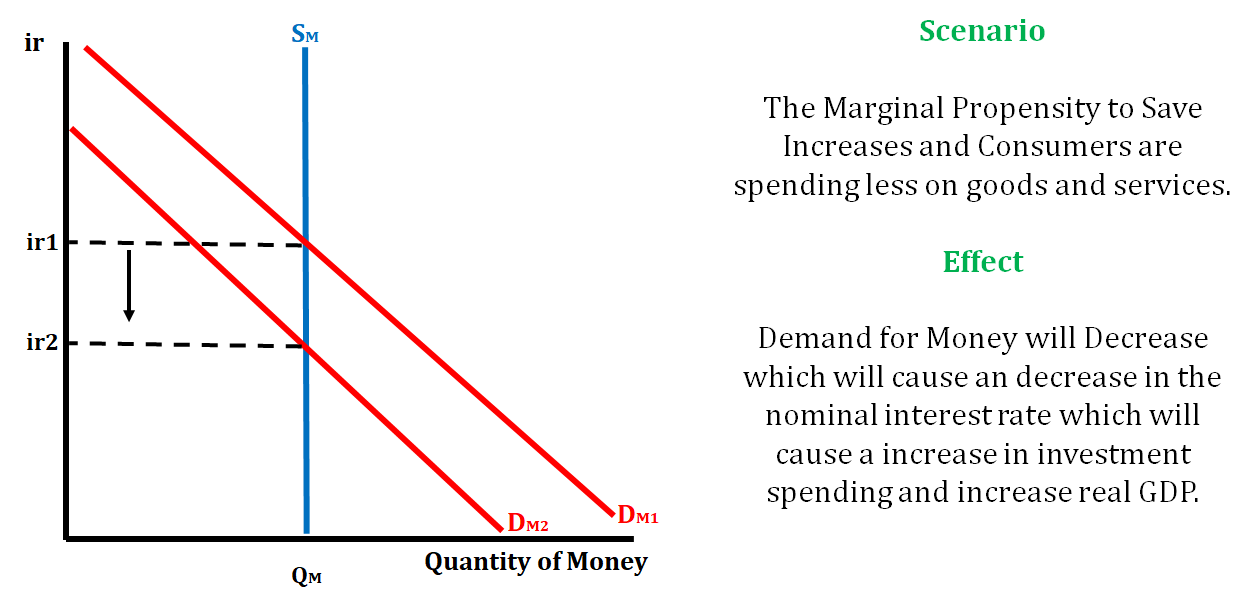
Let's look at the various ways that the money market equilibrium change through four different examples.
Example 1:
<br />
</p>
\
Example 2:
<br />
</p>
Example 3:
<br />
</p>
Example 4:
<br />
</p>
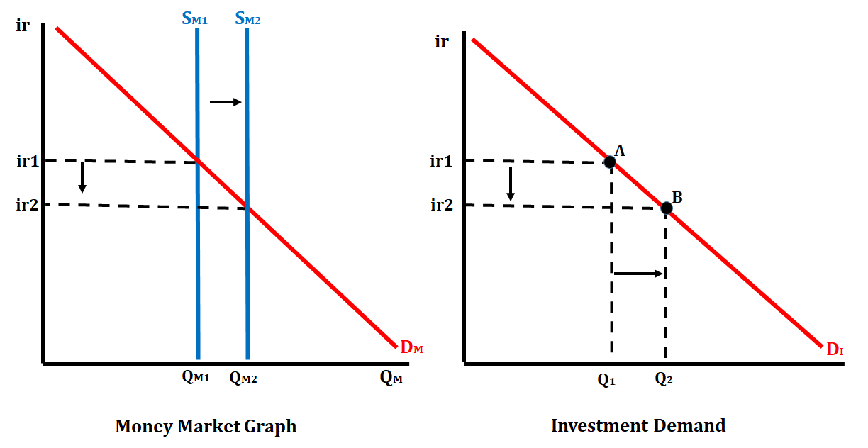
Investment Demand
It is the desired quantity of investment spending by firms across the economy on physical capital and other resources for the pe productivity/profitability.
There is an inverse relation between the nominal interest rate and the quantity of investment demanded.
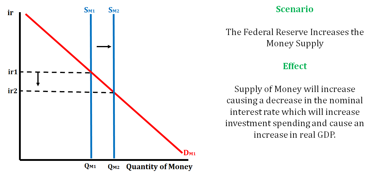
In the graph below, the Federal Reserve increases the money supply. This action will lower the nominal interest rate, and in turn, cause the quantity of investment demanded to increase.
<br />
</p>
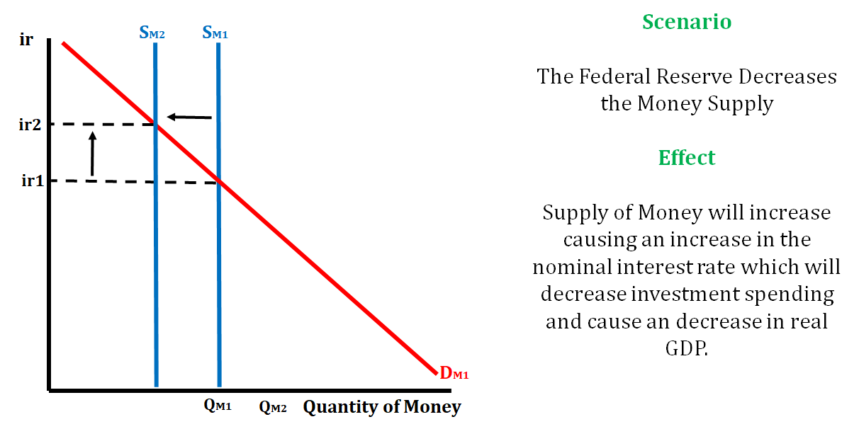
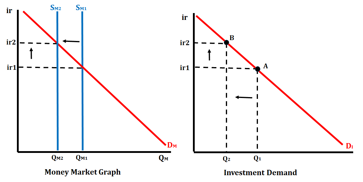
In the graph below, the Federal Reserve decreases the money supply. This action will raise the nominal interest rate, and in turn, cause the quantity of investment demanded to decrease.
<br />
</p>
4.6 Monetary Policy
Types of Monetary Policy
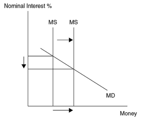
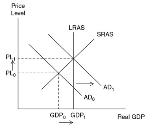
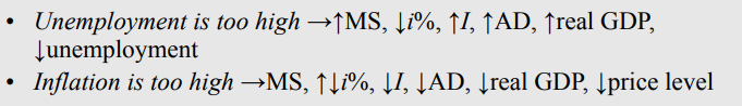
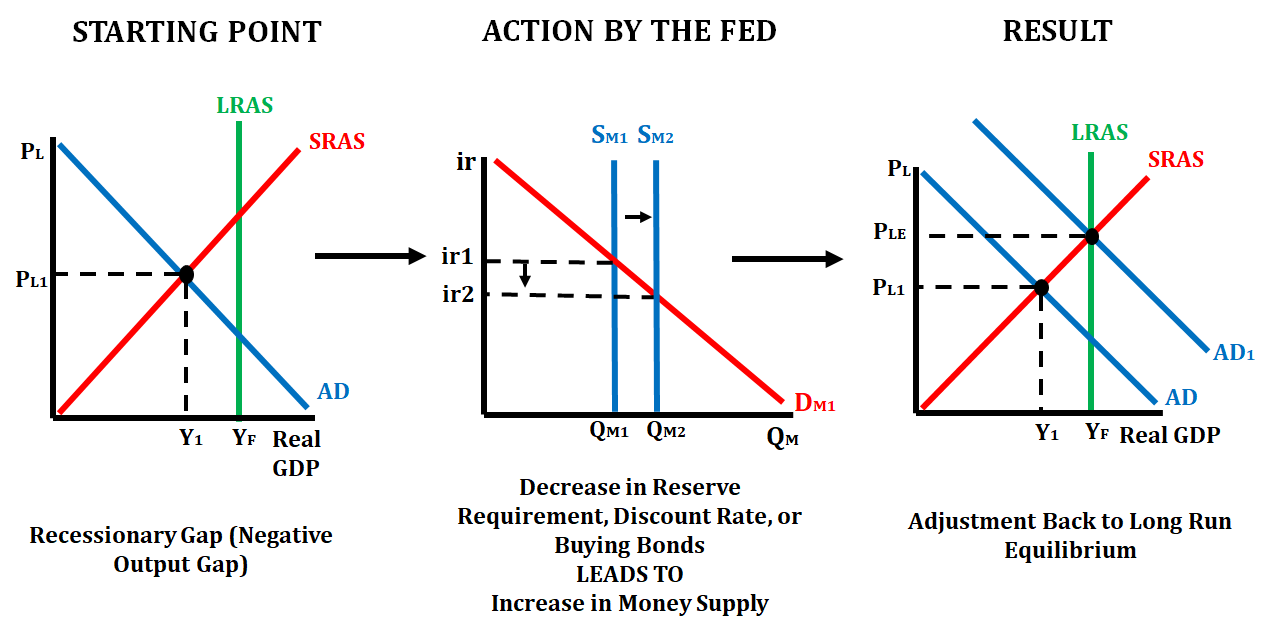
- Expansionary monetary policy - Designed to fix a recession by lowering interest rates to increase aggregate demand, lower the unemployment rate, and increase real GDP, which may increase the price level.
- By increasing the money supply, the interest rate gets lower. Lower interest increases private consumption and investments, which shifts the AD curve to the right.
\
\
\
\
\
\
\
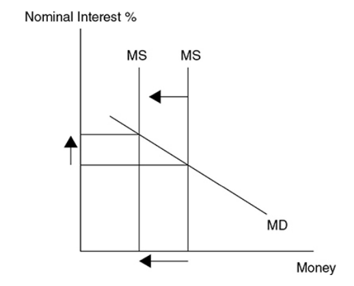
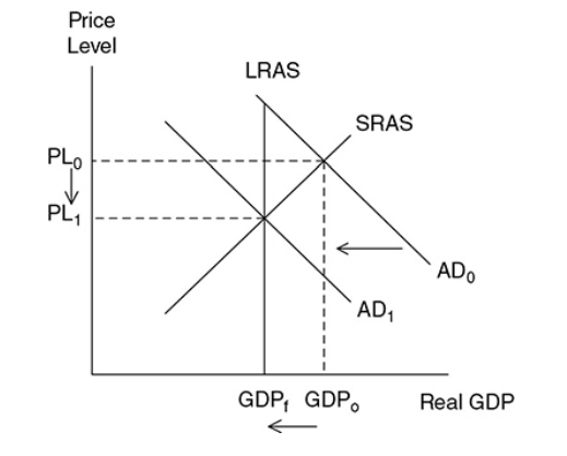
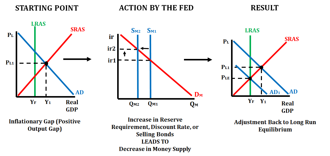
- Contractionary monetary policy - Designed to avoid inflation by increasing interest rates to decrease aggregate demand, which lowers the price level and decreases real GDP back to full employment.
- When the money supply is decreased, the interest rate increases causing a decrease in private consumption and investment shifting AD to the left.
\
\
\
\
\
\
\
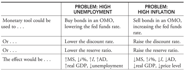
Tools of Monetary Policy
- Open market operations (OMOs) - A traditional tool of monetary policy, it involves the Fed’s buying (or selling) of securities from (to) commercial banks and the general public.
- When securities (Treasury bonds) are bought from the banks by the Fed, the banks receive excess cash and the Fed gets bonds. When banks have excess reserves, the money supply increases and the interest rate falls.
- When Fed buys, BB = BB → Buying Bonds = Bigger Bucks
- The opposite happens when the banks buy securities from the Fed. The banks get the bonds and their excess reserves would fall causing the money supply to decrease increasing interest rates.
- When Fed sells, SB = SB → Selling Bonds = Smaller Bucks
- Federal funds rate - The interest rate paid on short-term loans made from one bank to another. When this rate is a target for an OMO, bonds are bought or sold accordingly until the interest rate target has been met.
- If the FOMC wants to lower interest rates, it buys bonds.
- If the FOMC wants to rise interest rates, it sells bonds.
- Discount rate - The interest rate commercial banks pay on short-term loans from the Fed.
- Lowering the discount rate (or federal funds rate) increases excess reserves in banks and expands the money supply.
- Raising the discount rate (or federal funds rate) decreases excess reserves in commercial banks and contracts the money supply.
- Required Reserve Ratio -
- Lowering the reserve ratio increases excess reserves in commercial banks and expands the money supply.
- Increasing the reserve ratio decreases excess reserves in commercial banks and contracts the money supply.
\
\
\
4.7 The Loanable Funds Market
The demand of Loanable Funds
- It is the quantity of credit wanted and needed at every real interest rate by borrowers in an economy.
- The relationship between real interest rates and the number of loanable funds demanded is inverse.
Shifters for the demand of Loanable Funds
F = Foreign Demand for domestic currency
A = All Borrowing, Lending, and Credit
D = Deficit Spending
E = Expectations for the Future
</p>
Supply of Loanable Funds
- It is the quantity of credit provided at every real interest rates by banks and other lenders in an economy.
- The relationship between real interest rates and the quantity of loanable funds number is direct, or positive.
Determinants for the Supply of Loanable Funds
- S = Savings rate
- E = Expectations for the Future
- L = Lending at the Discount Window
- F = Foreign Purchases of Domestic Assets
\
Loanable Funds Market
- When borrowers and lenders come together, we refer to this as the loanable funds market.
Conclusion
- When the demand for loanable funds increases then the real interest rate will increase.
- When the demand for loanable funds decreases then the real interest rate will decrease.
- When the supply of loanable funds increases then the real interest rate will decrease.
- When the supply of loanable funds decreases then the real interest rate will increase
%%Unit 5: Long-Run Consequences of Stabilization Policies%%
5.1 Fiscal and Monetary Policy Actions in the Short-Run
Fiscal Policy
Classical Adjustment from Short-Run to Long-Run Equilibrium
- Adjustment to a recessionary gap:
\
\
\
\
- Based on this graph, the economy is currently operating at full employment. If consumers and firms begin to lose confidence in the labor market and overall economy, AD shifts to the left.
- In the short run, this causes a recessionary gap as real GDP falls to GDPr meaning that unemployment rises and aggregate price levels fall from PL1 to PL2.
- NOTE - One of the hallmarks of a recession is a decreased demand for many factors of production.
- This recessionary gap fixes itself since the prices of the products will decrease, causing a gradual rightward shift of the SRAS curve to SRAS2. The curve shifts to the right until the gap is closed and the economy is back at GDPf.
Adjustment to an inflationary gap:
<br />
</p>
\
- When the AD curve increases, an inflationary gap happens to cause an increase in real GDP to GDPi (lower unemployment rate) and an increase in the aggregate price level to PL2.
- When this happens, there’s stronger demand for labor and all of the other factors of production causing factor prices to rise. As the factor prices rise, the SRAS curve shifts to the left to SRAS2 eventually eliminating the inflationary gap, but at a higher aggregate price level of PL3.
Monetary Policy
Recessionary Gap Correction
\
\
Inflationary Gap Correction
\
\
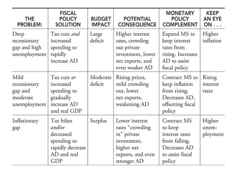
Coordination of Fiscal and Monetary Policy
- The central bank develops monetary policy and is independent of Congress and the president. This is a critical balance to fiscal policy that can be heavily politicized.
\
\
\
- In a deep recessionary gap, expansionary monetary policy could be used to assist expansionary fiscal policy in quickly moving to full employment. The risk then becomes a burst of inflation.
- In a mild recessionary gap, contractionary monetary policy could be used to offset expansionary fiscal policy to gradually move to full employment. The risk then becomes rising interest rates.
- In an inflationary gap, contractionary monetary policy could be used to assist contractionary fiscal policy to put downward pressure on the price level. The risk then becomes a rising unemployment rate.
5.2 Phillips Curve
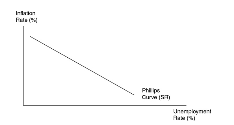
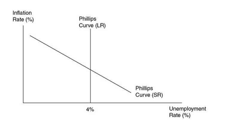
Phillips curve - A graphical device that shows the relationship between inflation and the unemployment rate. In the short run, it’s downward sloping, and in the long run, it’s vertical at the natural rate of unemployment.
- It shows the inverse relationship between inflation and the unemployment rate.
<br /> <br />
<br /> </p>
The possibility of deflation at extremely high unemployment rates means that the Philips curve may continue to fall below the x-axis.
Shifts in AD
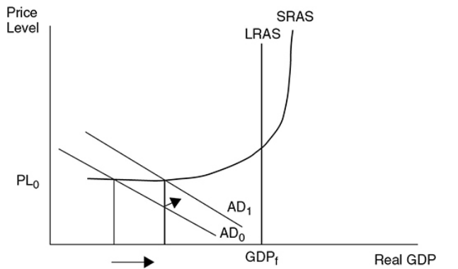
Demand-pull inflation - This inflation is the result of stronger consumption from all sectors of AD as it continues to increase in the upward-sloping range of SRAS.
If AD increases from AD0 to AD1 in the nearly horizontal range of SRAS, the price level may only slightly increase, while real GDP significantly increases and the unemployment rate falls.
<br /> <br />
<br /> </p>
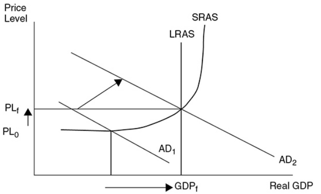
If AD continues to increase to AD2 in the upward-sloping range of SRAS, the price level begins to rise and inflation is felt in the economy.
<br /> <br />
<br /> </p>
If AD increases much beyond full employment to AD3, inflation is quite significant and real GDP experiences minimal increases.
<br /> <br />
<br /> </p>
Recession - In the AD and AS models, a recession is typically described as falling AD with a constant SRAS curve. Real GDP falls far below full employment levels and the unemployment rate rises.
Deflation - A sustained falling price level, usually due to severely weakened aggregate demand and a constant SRAS.
- If aggregate demand weakens, the opposite is expected. One of the most common causes of recession is falling AD since it lowers real GDP and increase the s unemployment rate. Deflation is expected here.
<br /> <br />
</p>
Shifting SRAS
Supply-side boom - When the SRAS curve shifts outward and the AD curve stays constant, the price level falls, real GDP increases and the unemployment rate falls.
The simplified
<br />
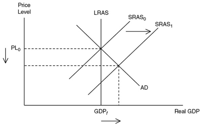
<br /> </p>
If nominal input prices fall, the SRAS curve shifts to the right.
Stagflation (Cost-push inflation) - A situation in the macroeconomy when inflation and the unemployment rate are both increasing. This is most likely the cause of falling SRAS while AD stays constant.
<br /> <br />
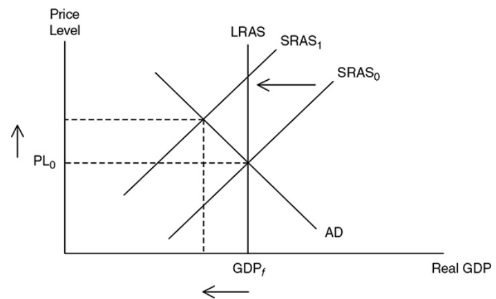
<br /> </p>
An increase in SRAS is the best possible macroeconomic situation. A decrease is one of the worst.
- A decrease creates inflation, lowers real GDP, and increases the unemployment rate.
The Long-Run Phillips Curve
The AS model assumes that the long-run AS curve is vertical and at full employment. This causes the Philips curve to be vertical at the natural rate of employment.
<br /> <br />
<br /> </p>
5.3 Money Growth and Inflation
Inflation
- It is the result of increasing the money supply.
- It closes the recessionary gap.
- In deflation:
- The money supply decreases.
- The inflationary gap will be closed.
- Price level will increase.
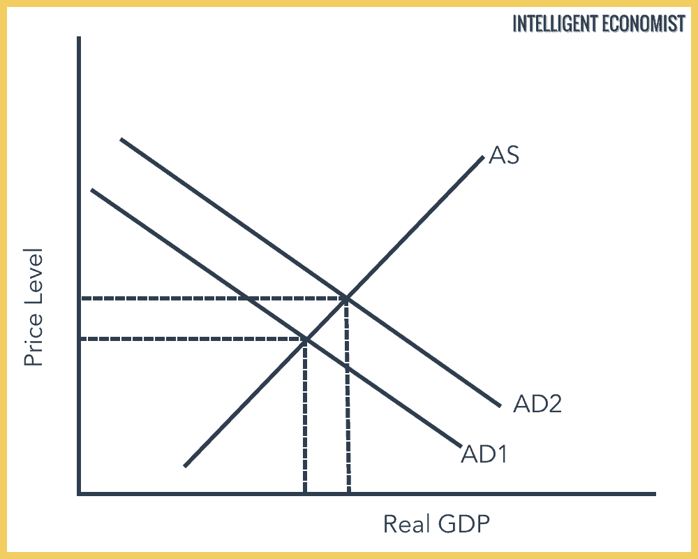
Demand-Pull Inflation
- It is caused by an increase in consumer demand.
- It happens when AD shifts to the right with consumers spending more.
- The price level increases.
- Real GDP increases.
- It is caused by too much government deficit spending.
- It usually drives up AD.
\
\
Seen in the graph above, AD1 shifts to the right to AD2, increasing both price and real GDP. This is also known as the inflationary gap, and it is corrected through long-run adjustment and contractionary fiscal or monetary policies.
</p>
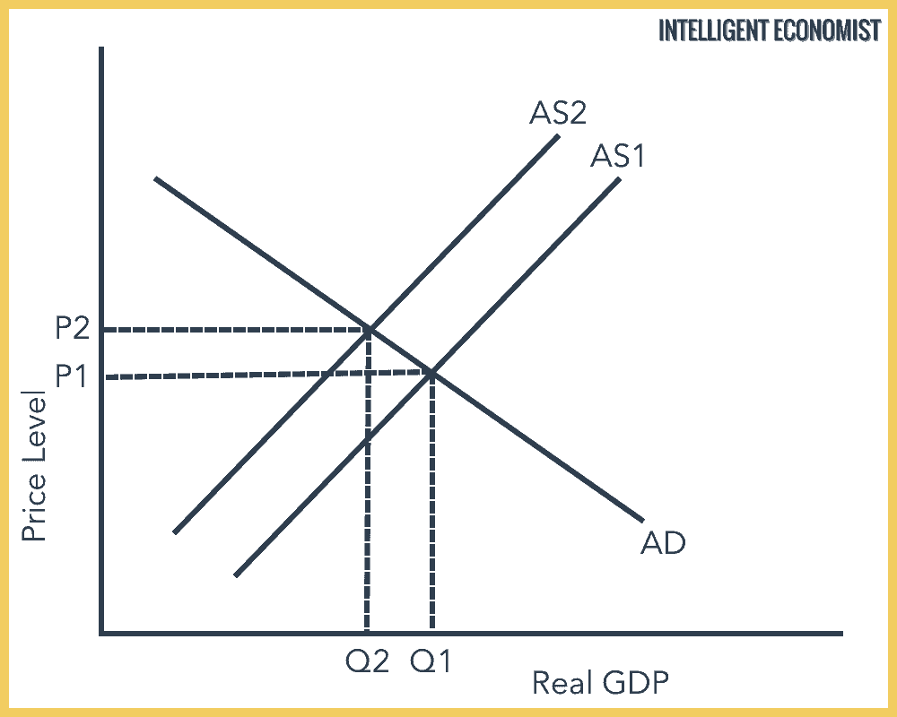
Cost-Push Inflation
- It is caused when production is decreased.
- Anything which disturbs production and decreases supply is to be cost-push inflation.
\
\
- With this type of inflation, supply shortages happen, leading to AS1 (short-run in this case) shifting to the left to AS2. This drives the price level to increase but the real GDP to decrease. This is a bad example of inflation because it's a little harder to fix.
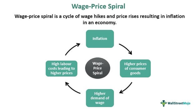
Wage-Price Spiral
- A self-perpetuating spiral where demand rises and supply goes down.
- Demand-pull and Cost-push are working together, which is the worst case with inflation.
\
\
- Everything is now at higher prices, which will lead to more inflation, then higher prices of everything, then higher demand for wages, then higher production costs, and it keeps going on.
\
\
As seen in the graph, we have a double shifter. AD is shifting to the right, while SRAS is shifting to the left. As a result, real GDP is unchanged, but we still have an increase in the price level.
Inflation due to Changes in the Money Supply
- Inflation can happen due to changes in monetary supply.
- Every time they increase or decrease the money supply, the price level can be indirectly affected.
- <br />
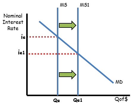
</p>
- MS, meaning money supply, was increased by the Fed. Consequently, the interest rate and quantity of money increased. This indirectly leads to an increase in price, thus inflation.
<br /> Theory of Monetary Equality
- A change in the money supply does not affect the economy.
- Only the dollar values are changed and nothing else.
- The theory of monetary neutrality is a nice way of saying money doesn’t matter.
</p>
The quantity theory of money - A theory that asserts that the quantity of money determines the price level and that the growth rate of money determines the rate of inflation.
It predicts that any increase in the money supply only causes an increase in the price level.
Equation of exchange - A way to view the quantity theory of money. The equation says that nominal GDP (P × Q) is equal to the quantity of money (M) multiplied by the number of times each dollar is spent in a year (V). MV = PQ.
The velocity of money - The average number of times that a dollar is spent in a year. V = PQ/M.
- Ex. → If in a given year the money supply is $100 and nominal GDP is $1,000, each dollar must be spent 10 times; V = 10.
If the money supply (M) increases, the increase must be reflected in the other variables. To accommodate an increase, the velocity of money must fall, the price level must rise, or the economy’s output of goods and services must increase.
Economists believe that the quantity of output produced in a given year is a function of technology and the supply of resources. Therefore, the increased money supply is going to only create inflation.
5.4 Deficits and the National Debt
Key Vocabulary
- Fiscal Stimulus—The use of expansionary fiscal policy, including an increase in government spending, a decrease in personal taxes, or an increase in income transfers.
- Fiscal Restraint—The use of contractionary fiscal policy, including a decrease in government spending, an increase in personal taxes, or a decrease in income transfers.
- Government Revenue—The total income gained by the government at all levels, through tax policies, including income taxes, excise taxes, and regulatory taxes.
- Government Expenditures—The total spending payments made by the government at all levels, including discretionary and non-discretionary purchases.
- Budget Surplus—The condition that exists when government revenues exceed government expenditures. This occurs when tax revenues are more than government purchases plus transfer payments in a given year.
- Budget Deficit—The condition that exists when government expenditures exceed government revenues. This occurs when tax revenues are less than government purchases plus transfer payments in a given year.
- National Debt—The accumulation of deficits over multiple years.
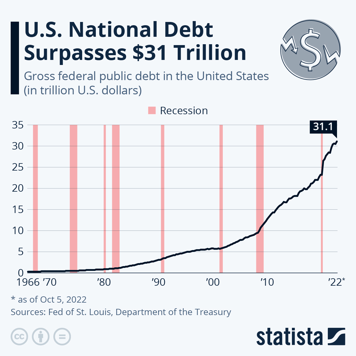
US National Debt
- The US government’s debt is immense.
- As of 2023, the debt is a huge $31 trillion!
\
\
Surplus and Deficit
- Surplus happens when the difference between tax revenues and government spending is positive.
- Deficit happens when the government spends more than its received revenue.
- The US government has three areas to spend a certain amount of money every year called mandatory spending.
- Social Security
- Medicare
- Interest on the national debt
State and Local Debts
- The US is operating in a recessionary gap, where tax revenues are low and spending is high, leading to a deficit.
- The US is operating in an expansionary gap, where tax revenues are high and spending low, leading to a surplus.
In both scenarios, if the Constitution required the state government to balance the budget to exactly zero here's what would happen:
- Government implements higher taxes and less spending, but this is a recipe for a recession!
- Government implements lower taxes and more spending, but this is a recipe for inflation!
5.5 Crowding Out
- Crowding out effect - It is the economic theory that public sector spending can lessen or eliminate private sector spending.
- The government’s budget deficit increases demand for loanable funds, but it reduces the number of available loan funds for private investors.
- Less investment happening by the private sector means national economic growth is not happening.
- This reduces demand and brings the economy back to where it started: a recessionary gap.
- Federal Government is the largest demander for loanable funds.
\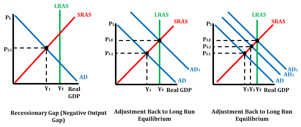
\
- The graph on left shows an economy in a recessionary gap.
- The graph in middle shows the rightward shift of aggregate demand.
- It can correct a recessionary gap when the government increases its spending.
- The graph on the right shows what can happen when crowding out occurs.
- Instead of government spending correcting the economy, they choose to spend money on a good or service that will decrease or eliminate private spending, causing the economy to move only from AD to AD2. When crowding out occurs, the economy does not quite get back to long-run equilibrium.
Long-Run Impact
- Crowding out is not always an issue.
- Sometimes, there will be enough loanable funds for everyone.
- The government borrows loanable funds but siit its is already in deficit the situation just worsens and turns into a looming depression.
- Economy:
- Crowding out prolongs -
- economic growth reduced.
- economy might start going downhill
- widen the recessionary gap.
- finally results in economic doom.
- Infrastructure:
- Crowding out prolongs -
- private investments decrease.
- low investments leads to a decrease in inefficiency in building things.
5.6 Economic Growth
GDP per capita
Growth is measured through real GDP per capita.
GDP per capita = real GDP / population
If GDP per capita increases, economy grew.
</p>
Aggregate Production Function
- The aggregate production function is a function that shows the relationship between production and capital.
- It shows long-run economic growth.
Production Possibilities
\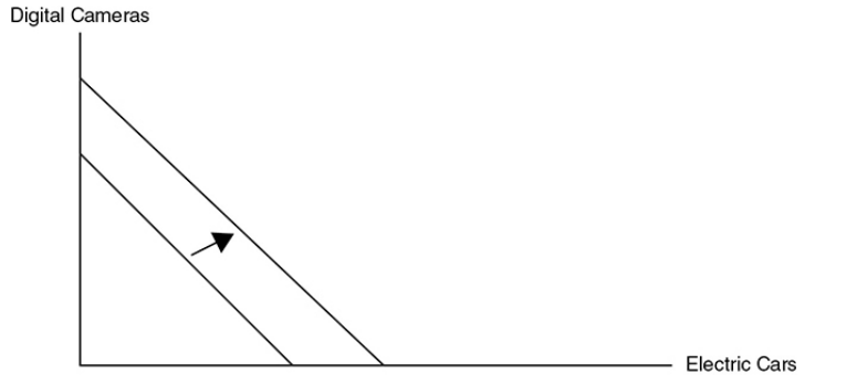
\
\
- This graph shows that the country’s production possibilities in electric cars and digital cameras grows over time if
- The quantity of economic resources increases,
- The quality of those resources improves.
- The nation’s technology improves.
Productivity
- Productivity - The quantity of output that can be produced per worker in a given amount of time.
- If the labor force of a country produces more output per worker from one year to the next, productivity has increased and the PCC shifted outwards.
Determinants of Productivity
- All of these require an investment, funds that come from savings. Firms invest in physical capital and individuals invest in human capital. Countries invest in natural resources entrepreneurs invest in technology.
- Stock of physical capital - When the quantity of physical capital in an economy is increased, in many cases, the capital helps increase the quantity of more capital.
- Human capital - The amount of knowledge and skills that labor can apply to the work that they do and the general level of health that the labor force enjoys.
- Natural resources - Productive resources provided by nature.
- Nonrenewable resources - Natural resources that cannot replenish themselves. Coal is a good example.
- Renewable resources - Natural resources that can replenish themselves if they are not overharvested. Lobster is a good example.
- Technology - A nation’s knowledge of how to produce goods in the best possible way.
5.7 Public Policy and Economic Growth
Public Policy
- Types of Public Policy:
- Increase in education spending
- By increasing investment in the education of workers, those workers are more effective and can produce more. Improving human capital increases the quality of labor available, which causes an increase in economic growth.
- Increase in infrastructure spending
- For example, if the government sets up dependable transportation systems, then they are helping businesses get inputs to production, and get goods to customers. This means that government spending on infrastructure raises government spending and contributes to the growth of real GDP in the long run.
- Policies that spur innovation
- By creating policies that promote innovation, the government can promote economic growth in the long run. For example, the government can create policies that protect intellectual property (patents), which would give private companies a greater incentive to create that intellectual property. By promoting creativity and entrepreneurship, we will be able to increase real GDP in the long run.
- Increasing employment
- By increasing employment, more workers will lead to increased productivity, thus leading to economic growth.
Supply-Side Policies
- Supply-side fiscal policy - Fiscal policy centered on tax reductions targeted to AS so that real GDP increases with very little inflation.
- The main justification is that lower taxes on individuals and firms increase incentives to work, save, invest, and take risks.
Saving and Investment
Investment tax credit - A reduction in taxes for firms that invest in new capital like a factory or piece of equipment.
<br /> <br />
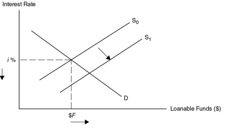
<br /> </p>
Lower income taxes create disposable income for households, increasing both consumption and savings from households and the profitability of investment for firms. This allows for an increase in the productive capacity of the country because more capital stock is accumulated. As well, this increases the long-run AS curve. Tax incentives to increase savings and investment are likely to increase AD.
\
\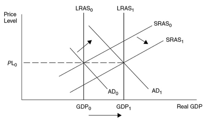
\
\
How lower taxes can increase AS and AD
Productivity incentives - Lower taxes mean workers take more of their pay home, which might prompt wage earners to work harder, take less time off, and be more productive.
Risk-taking - Lowering the tax rate on profits increases the expected rate of return and encourages more investment.
</p>
%%Unit 6: Open Economy—International Trade and Finance%%
6.1 Balance of Payment Accounts
Balance of Payments Accounts
- Balance of payments statement - A summary of the payments received by the United States from foreign countries and the payments sent by the United States to foreign countries.
Current Account
Current account - This account shows current import and export payments of both goods and services and investment income sent to foreign investors of the United States and investment income received by U.S. citizens who invest abroad.
- Ex. → If a Canadian is receiving dividends from an American corporation or interest from a U.S. Treasury bill, these dollars would be sent out of the country.
- A deficit balance tells us that the United States sent more American dollars abroad than foreign currency received in current transactions.
<br /> <br />
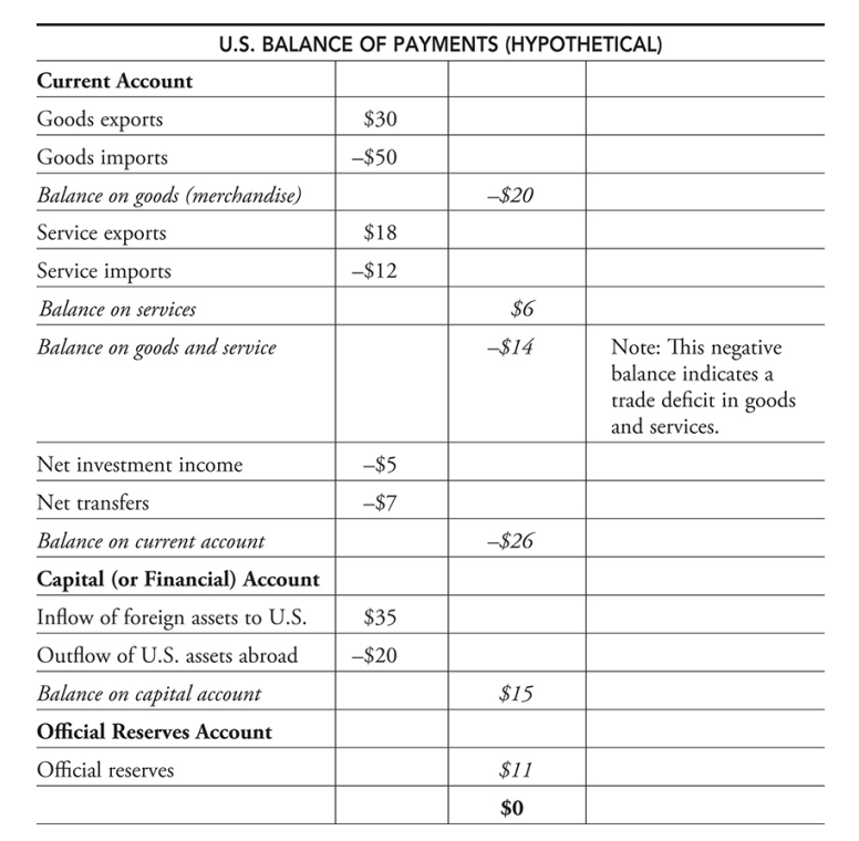
</p>
Capital (or Financial) Account
- Capital (or financial) account - This account shows the flow of investment on real or financial assets between a nation and foreigners.
- Ex. → If a Swedish firm buys a manufacturing facility in Idaho, or if a Mexican citizen buys a U.S. Treasury bond, it is recorded as an inflow of foreign capital assets into the United States.
- A surplus balance tells us that there was more foreign capital investment in the United States than there was U.S. investment abroad.
Official Reserves Account
- Official reserves account - The Fed’s adjustment of a deficit or surplus in the current and capital account by the addition or subtraction of foreign currencies so that the balance of payments is zero.
- Balance of payments deficit - When the US has sent more dollars out than foreign currency has come in while adding the current and capital account. When this happens, the Fed credits the account to balance it.
- Balance of payment surplus - When more foreign currency was coming into the US than American dollars sent abroad. Here, the Fed transfers the surplus currency bank into official reserves.
A Circular Flow of Dollars
- The U.S. dollars that Americans send to foreigners are equal to the U.S. dollars that foreigners send to Americans.
- If Americans import more goods and services from abroad, the current account will move in the deficit direction but the capital/financial account will move in the surplus direction as those dollars return.
6.2 Exchange Rates
Currency Markets
Exchange rate - The price of one currency in terms of a second currency.
- Ex. → If 2 dollars = 1 euro, 1 dollar = 0.5 euro.
<br /> <br />
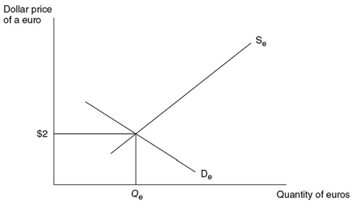
</p>
Changes in Exchange Rate
- Determinants of exchange rates - External factors that increase the price of one currency relative to another.
- Consumer tastes - When domestic consumers build a stronger preference for foreign-produced goods and services, the demand for those currencies increases and the dollar depreciates. If foreign consumers increase their demand for U.S.-made goods, the dollar appreciates.
- Relative incomes - When a nation’s macroeconomy is strong and incomes are %%r%%ising, they increase their demand for all goods, including those produced abroad.
- Ex. → If Europeans are enjoying economic growth and the United States is in a recession, the relative buying power of European citizens is growing, meaning that the consumption of domestic and U.S.-made goods increases demand for the dollar appreciating its value.
- Speculation - Foreign currencies can be traded as assets causing investors to seek to profit from buying currency at a low rate and selling it at a higher rate.
- Ex. → If it appears that future interest rates will fall in the United States relative to interest rates in Japan, the yen seems like a good investment. Speculators would then increase their demand for Japanese assets, thus appreciating the yen and depreciating the dollar.
6.3 Foreign Exchange Market
Foreign Exchange Demand
- It is the quantity of an international currency that all domestic and foreign currencies are willing and able to purchase at various rates of exchange.
- The relationship between exchange rates and the quantity of currency demanded is inverse:
- As the exchange rate rises, domestic and foreign consumers will purchase less quantity of the currency.
- As the exchange rate falls, domestic and foreign consumers will purchase more quantity of the currency.
\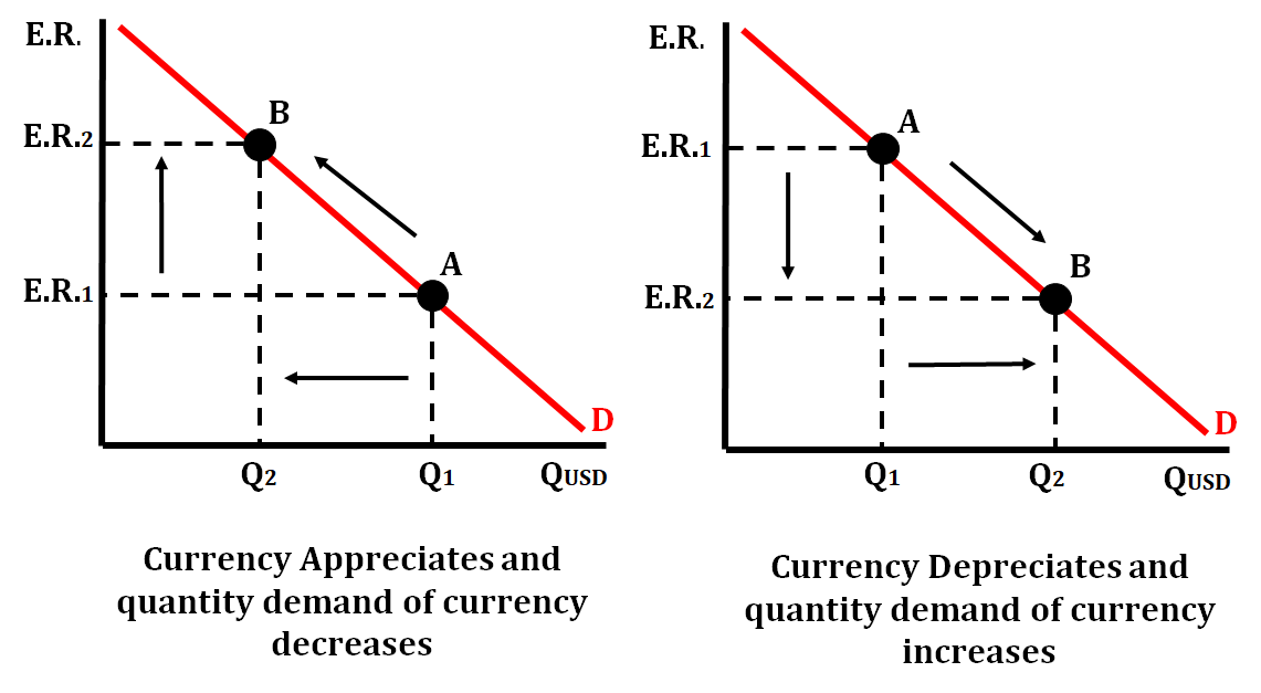
\
Foreign Exchange Supply
- It is the quantity of an international currency that all domestic and foreign sellers are willing and able to sell at various rates of exchange.
- The relationship between exchange rates and the quantity of currency supplied is positive or direct:
- As exchange rates rise, domestic and foreign consumers are willing to sell more.
- As exchange rates fall, domestic and foreign consumers are willing to sell less.
\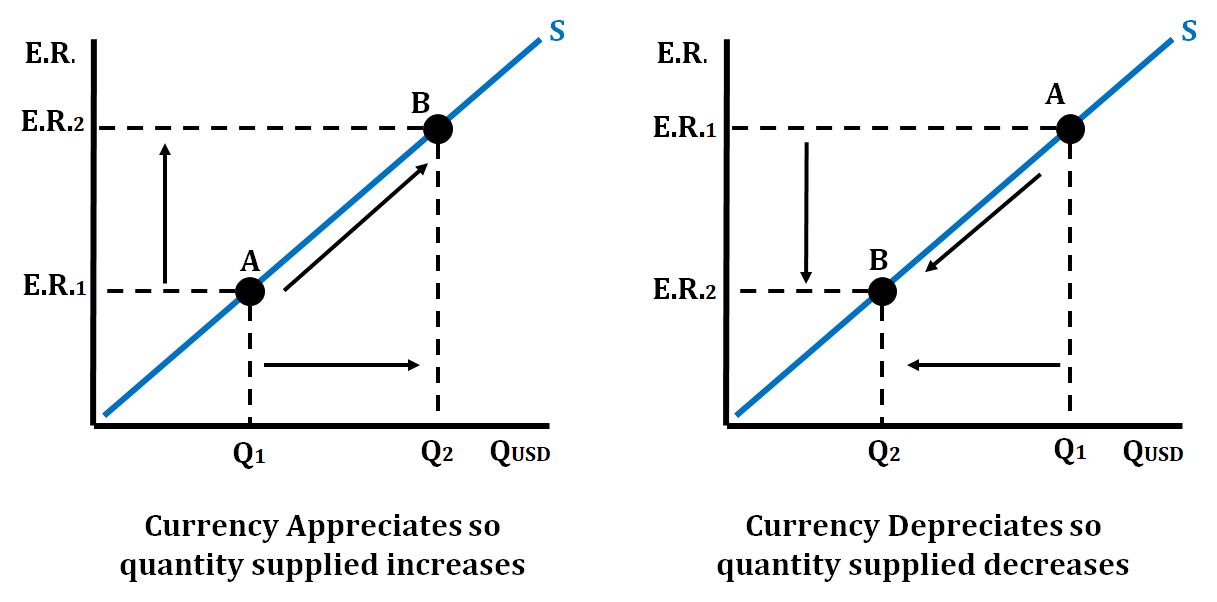
\
FOREX Market Equilibrium
- It is achieved in the FOREX Market (the market in which foreign currency is bought and sold) when the quantity supplied of the currency equals the quantity demanded of the currency at a specific exchange rate.
- The FOREX Market in equilibrium for EURO and U.S. Dollar
\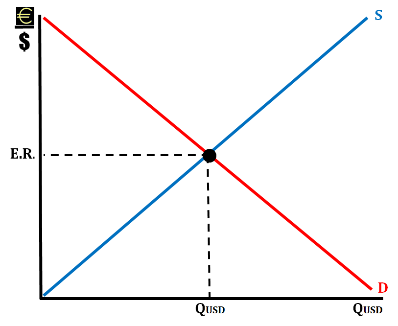
\
Connection to Monetary Policy
- . When the Fed increases the money supply, the interest rates on American financial assets begin to fall, so the demand for the dollar falls and it depreciates relative to other foreign currencies.
- This makes goods in the US less expensive to foreign consumers, so American net exports increase shifting AD to the right.
- If the Fed decreases the money supply, American interest rates begin to rise and the dollar appreciates relative to foreign currencies.
- This makes American goods more expensive decreasing the net exports which shift AD to the left.
- When interest rates rise, capital investments decrease, and financial investments increase.
\
\
\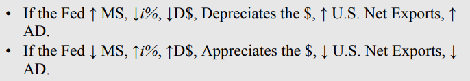
\
- Demand for the U.S. dollar increases and the dollar appreciates relative to the euro if:
- European taste for American-made goods is stronger.
- European relative incomes are rising, increasing demand for U.S. goods.
- The U.S. relative price level is falling, making U.S. goods relatively less expensive.
- Speculators are betting on the dollar to rise in value.
- The U.S. relative interest rate is higher, making the United States a relatively more attractive place for financial investments.
6.4 Effect of Changes in Policies & Economic Conditions on the Foreign Exchange Market
Change in Demand or Supply in Currency
- There are four determinants that can change Four determinants canOREX Market.
- Foreign tastes
- Trade prices
- Income levels
- Real interest rates
Fiscal Policy Impact on Exchange Rates
- When the government practices an expansionary fiscal policy (increase in spending or decrease in taxes), there is an effect on the exchange rate for that country's currency.
- If the government increases spending or decreases taxes, aggregate demand will increase, GDP increase, and price increase.
\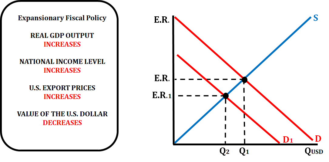
\
- When the government practices a contractionary fiscal policy (decreases spending or increases taxes), there is an effect on the exchange rate of that country's currency
- If the government decreases spending or increases taxes, aggregate demand will decrease, GDP decrease, and price decrease.
\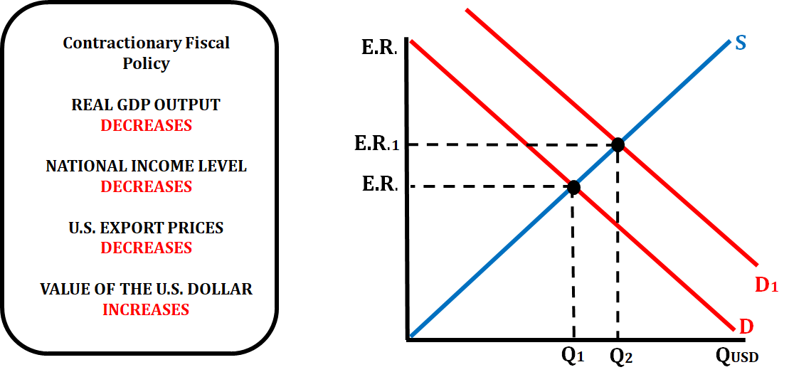
\
Monetary Policy Impact on Exchange Rates
- If the central bank of a country is practicing an expansionary monetary policy (decreasing the reserve ratio, decreasing the discount rate, or buying bonds) it will affect the exchange rate as well.
- When the FED increases the money supply, that lowers the interest rate which will increase investment spending.
- When investment spending increases, aggregate demand increases which raises the price level.
- This means that both the national income levels and export prices will increase.
\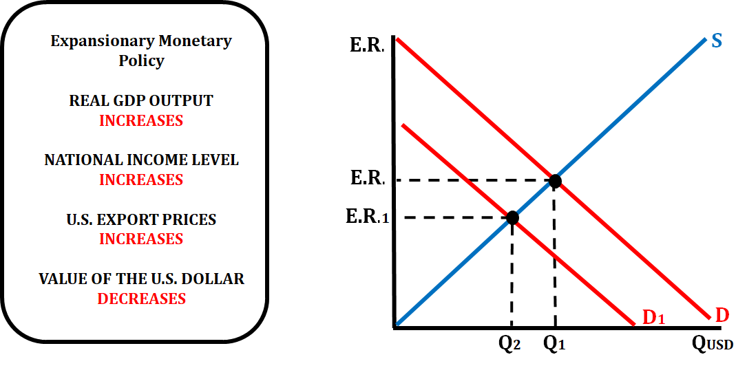
\
- If the central bank of a country is practicing a contractionary monetary policy (increasing the reserve ratio, increasing the discount rate, or selling bonds), it will affect the value of the exchange rate.
- When the FED decreases the money supply, that raises the interest rate which will decrease investment spending.
- When investment spending decreases, aggregate demand decreases which lower the price level.
- This means that both the national income levels and export prices will decrease.
\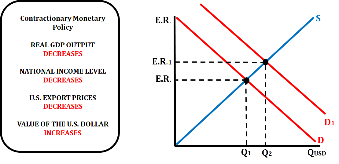
\
Tariffs
- Revenue tariff - An excise tax levied on goods not produced in the domestic market.
- Ex. →The United States does not produce bananas. If a revenue tariff were levied on bananas, it would not be a serious impediment to trade, and it would raise a little revenue for the government.
- Protective tariff - An excise tax levied on a good that is produced in the domestic market so that it may be protected from foreign competition.
- Ex. → Assume the domestic steel price is $100 per ton and the equilibrium quantity of domestic steel is 10 million tons. Since other nations could produce it at a lower cost, in the competitive world market, the price is $80 per ton. At that price, the United States would demand 12 million tons but only produce eight million tons and so four million tons are imported. If the steel industry is successful in getting a protective tariff passed through Congress, the world price rises by $10, increasing the quantity of domestic steel supplied and reducing the amount of steel imported from four million to two million tons.
- A higher price and lower consumption reduce the area of consumer surplus and create deadweight loss.
\
\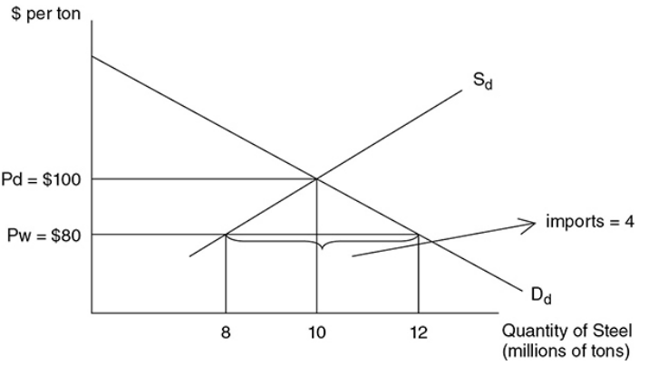
\
\
Economic Effects of the Tariff
- Consumers pay higher prices and consume less steel
- Consumer surplus has been lost
- Domestic producers increase output
- Domestic steel firms are not subject to the tariff, so they can sell more steel at the price of $90 than they could at $80.
- Declining imports
- Fewer tons of imported steel arrive in the United States.
- Tariff revenue
- The government collects $10 × 2 million = $20 million in tariff revenue. This is a transfer from consumers of steel to the government, not an increase in the total well-being of the nation.
\
\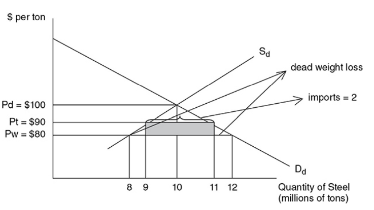
\
\
- Inefficiency
- The world price was lower than the domestic price because it was more efficient to produce steel abroad and export it to the United States. By taxing this efficiency, the United States promotes the less efficient domestic industry and stunts the efficient foreign sector. As a result, resources are diverted from the efficient to the inefficient sector.
- The deadweight loss now exists
Quotas
- Import quota - A limitation on the amount of a good that can be imported into the domestic market.
- With a quota, the government only allows two million tons to be imported. So the impact of the quota, except the revenue, is the same: higher consumer price and inefficient resource allocation.
\
\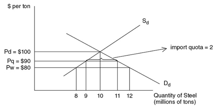
\
\
- Tariffs and quotas share some of the same economic effects:
- Both hurt consumers with artificially high prices and lower consumer surplus.
- Both protect inefficient domestic producers at the expense of efficient foreign firms, creating a deadweight loss.
- Both reallocate economic resources toward inefficient producers.
- Tariffs collect revenue for the government, while quotas do not.
6.5 Changes in the Foreign Exchange Market and Net Exports
Appreciating and Depreciating Currency
- Appreciating or stronger currency - When the value of a currency is rising relative to another currency.
\
\
\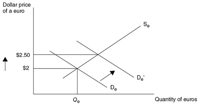
\
\
\
- Depreciating or weaker currency - When the value of a currency is falling relative to another currency.
\
\
\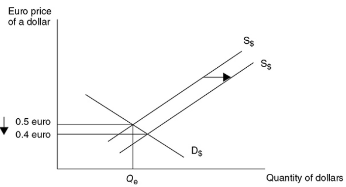
\
\
\
- NOTE - It is very important to label the axes correctly. If the market is for the dollar, the x-axis should be labeled “Quantity of dollars.” The label on the y-axis depends on how the dollar is being priced. If we are pricing dollars in terms of the number of euros it takes to purchase 1 dollar, then the correct label is “Euros per dollar” or “Euro price of a dollar”.
Changes in Net Export: Consequences
- Changes in net export can bring significant impact.
- Decrease in net exports:
- decrease in aggregate demand.
- exports become more expensive.
- decrease in demand for domestic goods.
- decrease in production and employment.
- decrease in output.
- Increase in net exports:
- increase in aggregate demand.
- exports become cheaper.
- increase in demand for domestic goods.
- increase in production and employment.
- increase in output.
6.6 Real Interest Rates and International Capital Flows
Capital Flow
- Inbound capital flow
- It is the injection of funds into a domestic economy that occurs through the purchase of domestic assets by foreign investors.
- When real interest rates are high, it generates inbound capital flow.
- This is because foreign investors look to invest their money into assets that have high-interest rates because they can earn a higher profit.
Outbound capital flow
- It is the extraction of funds from a domestic economy that occurs through the purchase of foreign assets by domestic investors.
- When real interest rates fall, it generates outbound capital flow.
- This is due to the foreign investors look to invest in other countries because the interest rate is higher there than in their own country.
Impact on net exports
A higher real interest rate in one country compared to another will make the currency of the country with the higher interest rate more attractive to foreign investors, leading to an appreciation of that currency. This can make exports from the country with the higher interest rate more expensive for foreign buyers, and imports to that country cheaper, which can lead to a decrease in net exports.
On the other hand, a lower real interest rate in one country compared to another will make the currency of the country with the lower interest rate less attractive to foreign investors, leading to a depreciation of that currency. This can make exports from the country with the lower interest rate cheaper for foreign buyers, and imports to that country more expensive, which can lead to an increase in net exports.
Central Banks and Domestic Interest Rates
- Central Banks
- It plays a major role in determining domestic interest rates.
- It uses monetary policy tools such as open market operations, discount rates and reserve requirements to influence interest rates.
- When the central bank raises the interest rate, it will encourage banks to raise their own interest rates as well.
- Domestic Interest Rates
- Affects net capital inflows:
- country’s assets become more or less attractive to foreign investors.
- domestic interest rate high → foreign investors may be likely to invest.
- domestic interest rate low → foreign investors may be less likely to invest.
- Banks affect domestic interest rates:
- When banks raise the interest rates they charge on loans, it can lead to higher borrowing costs for businesses and consumers, which can, in turn, lead to higher interest rates across the economy.
- When banks raise the interest rates they pay on deposits, it can lead to higher returns for savers, which can encourage them to save more and spend less, which can also lead to higher interest rates across the economy.
\