Macroeconomics
AP Macroeconomics
Unit 1: Basic Economic Concepts
Gourishankar Residential English Medium School
scarcity
factors of production
organizations of society
opportunity costs and trade-offs
the production possibility curve
efficiency
growth
comparative advantage and trade
demand
supply
market equilibrium


Unit 1: Basic Economic Concepts
Let’s have a quick overview of what economics is all about!
Economics
The study of how people, firms, and societies use their scarce productive resources to best satisfy their unlimited material wants.
It is the systematic study of choice.
In the realm of economics, all resources around us are considered to be limited; even the most basic things which exist around us like air or water.
Now, having an overall idea of what economics is all about. It’s time to dive into some crucial concepts:
1.1 Scarcity
All factors of production are scarce; therefore, the production of goods and service are also scarce.
The economic problem states however that our needs our unlimited and as mentioned earlier, the resources available are scarce.
Macroeconomics V/s Microeconomics
Macroeconomics: with macroeconomics, we consider the big picture- the nation’s economy as a whole. E.g., would changes to the money supply have an effect on country A’s imports and export?
Microeconomics: microeconomics filters our scope to individuals in an economy while keeping the overall economy in mind.
Resources or Factors of Production
Labor - Human effort and talent, physical and mental. This can be augmented by education and training (human capital).
Land or natural resources - Any resource created by nature. This may be arable land, mineral deposits, oil and gas reserves, or water.
Physical capital - Human-made equipment like machinery as well as buildings, roads, vehicles, and computers.
Entrepreneurial ability - The effort and know-how to put the other resources together in a productive venture.
Opportunity Costs and Trade-offs
Opportunity cost - The value of what was given up.
Ex. → If you use a scarce resource to pursue activity X, the opportunity cost of activity X is activity Y, the next best use of that resource.
Ex. → You have one scarce hour to spend between studying for an exam or working at a coffee shop for $8 per hour or mowing your uncle’s lawn for $10 per hour. If you choose to study, what is the opportunity cost of studying?
The opportunity cost of using your resource to do activity X is the value the resource would have in its next best alternative use. Therefore, the opportunity cost of studying is $10, the better of your two alternatives.
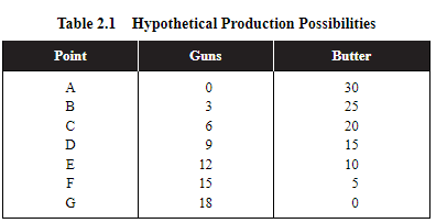
Calculations:
The opportunity cost for guns (D):
(20-15) - (9-6) = (5/3) = 1.67
The opportunity cost for butter (D):
(12-9) - (15-10) = (3/5) = 0.6
Trade-Offs
Since we have scarce resources, individuals, firms, and governments are faced with trade-offs.
Some examples of trade-offs for individuals are choosing between housing arrangements, transportation options, grocery store items, etc.
For firms, the trade-offs are often centered on which good or service can be provided, how much should be produced, and how to go about producing those goods and services.
The government is faced with issues that are likely to have an immediate impact on the lives of local citizens.
1.2 Opportunity Cost and the Production Possibilities Curve (PPC)
Production Possibilities Curve
To examine production and opportunity cost, economists find it useful to create a simplified model of an individual, or a nation, that can choose to allocate its scarce resources between the production of two goods or services.
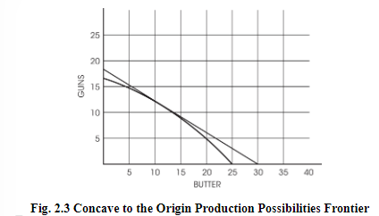
Realistically, PPC curves are not straight lines and tend to be concave-shaped.
The reason for this concave shape is that certain resources are more compatible with the production of a specific good/service.
Thus, when they are used up forcefully, they are less productive-hence the higher opportunity cost arises.
A generalized view of the production possibility curve:
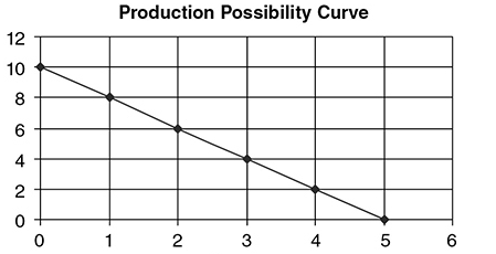
The slope of the curve measures the opportunity cost of the good on the x-axis.
The inverse of the slope measures the opportunity cost of the good on the y-axis.
Constant Opportunity Cost v/s Increasing Opportunity Cost
The production possibilities curve can illustrate two types of opportunity costs:
Increasing opportunity costs:
We must weigh the benefits and costs of our choices.
Opportunity cost is the cost of the next best alternative that we must give up pursuing a certain action.
For instance, if we have $10 and we choose to buy coffee for $2, the opportunity cost is the pastry we could have purchased instead.
The opportunity cost increases with every decision we make, as we give up more alternatives. This is called increasing opportunity cost.
It's crucial to consider the opportunity cost of each decision to make the most efficient use of our resources and maximize our benefits.
Decreasing opportunity costs:
To decrease opportunity costs, increase efficiency by using fewer resources to achieve the same output.
Prioritize important goals and allocate resources towards them to minimize the opportunity cost of not pursuing other goals.
Increase flexibility by adapting quickly to changing circumstances and being open to new ideas.
The graph for decreasing opportunity curve is not possible in real life.
Efficiency
Productive efficiency - When the economy is producing the maximum output for a given level of technology and resources. All points on the production frontier are productively efficient.
Allocative efficiency - The economy is producing the optimal mix of goods and services.
Optimal - The combination of goods and services that provides the most net benefit to society.
Market failure - When a market fails to produce the allocative efficient quantity.
Growth
Economic growth - The ability to produce a larger total output over time. Can occur if one or all of these happen:
An increase in the number of resources.
An increase in the quality of existing resources.
Technological advancements in production.
Economic contraction - It is when a country's economy shrinks due to factors such as reduced spending by consumers, businesses, or the government.
Economic contractions are a normal part of the business cycle and can lead to long-term growth if managed correctly.
1.3 Comparative Advantage and Trade
Comparative Advantage and Specialization
Absolute advantage -
The absolute advantage is producing goods/services more efficiently, using fewer inputs.
Let’s say a bakery and a pizza parlor both produce pizza crusts and pastries.
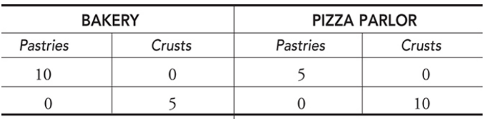
This graph presents the number of pastries and crusts each shop can produce. Since the bakery can produce more pastries than the pizza parlor, the bakery has an absolute advantage in pastry production.
Comparative advantage -
In macroeconomics, this principle is the basis for showing how nations can gain from free trade. Using the same example as before, we can say that the bakery has a comparative advantage since it can produce pastries at a lower opportunity cost. In the same way, the pizza parlor has a comparative advantage in pizza crusts.
They describe the way that individuals, nations, and societies can acquire more goods at a lower cost.
There are two types of problems:
Output problems:
To determine the absolute advantage, you are simply looking for which country can produce a higher amount of goods or services.
To determine you have to calculate per unit opportunity cost using the formula give up/gain (the amount of good you are giving up divided by the amount of good you are gaining). Once you have calculated per unit opportunity cost, the country with the lowest one has a comparative advantage.
If the two countries can both make the same amount of the good, then we say neither country has an absolute advantage.
Countries export what they have a comparative advantage in and import what they don't have a comparative advantage in.
Input problems:
To determine absolute advantage, you are looking for the country that uses the least number of resources (i.e., the lower number).
To determine comparative advantage, you have to calculate the per unit opportunity cost using the formula gain/give up. Once you have calculated the per unit opportunity cost the country with the lowest one has a comparative advantage.
If the two countries can both make one unit of the good with the same number of resources, then we say neither country has an absolute advantage.
Countries export what they have a comparative advantage in and import what they don't have a comparative advantage in.
Terms of trade:
It deals with the country’s export prices to income prices and determines the relative price between the nation’s exports and imports.
1.4 Demand
Law of demand - Holding all else equal, when the price of good rises, consumers decrease the quantity demanded of that good.
All else equal - To predict how a change in one variable affects a second, we hold all other variables constant. This is also referred to as the ceteris paribus assumption.
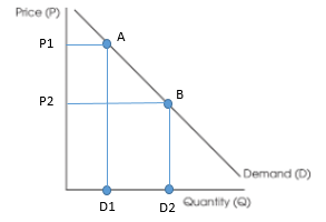
Change in Quantity Demanded vs. Change in Demand
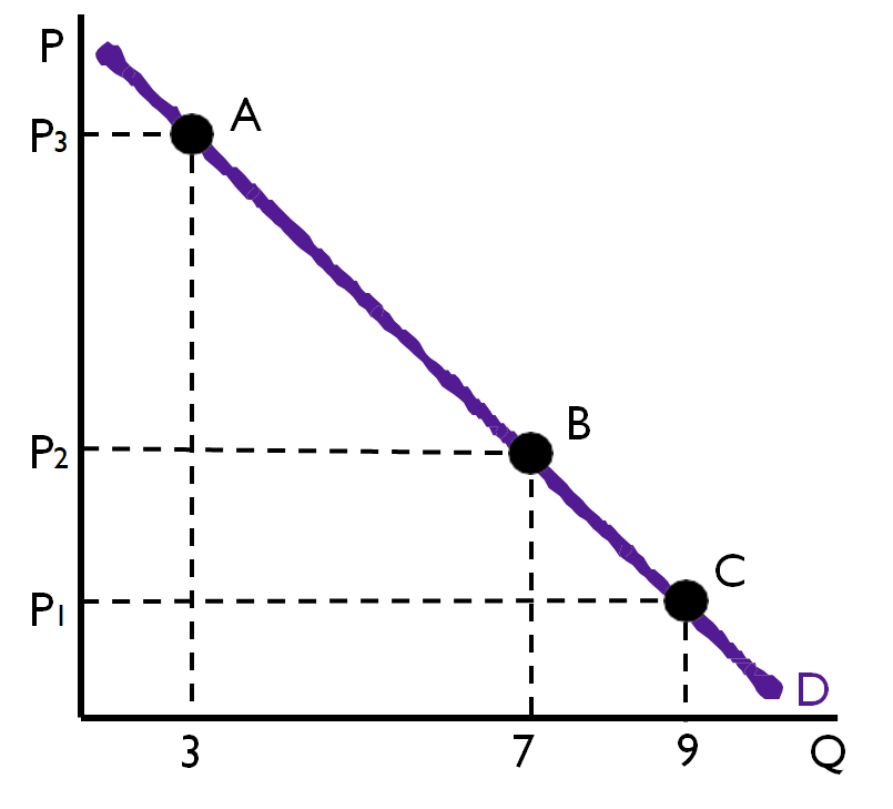
Change in the quantity demanded only occurs due to change in price-movement along the curve.
If product A would become expensive (P2 to P1), the quantity demanded would fall (D2 toD1)
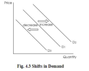
Changes in demand are when the entire curve would shift upwards or downwards.
These are the determinants of demand which are variables causing consumers to buy more or less of a product, irrespective of the price.
Determinants of Demand
The INSECT Acronym:
I = Income:
Goods are usually categorized into 2 types, inferior and normal.
Demand tends to decline (shift downwards) for inferior goods with an increase in consumer income.
Demand for normal goods increases (shifts upwards) with an increase in consumer income.
N = Number of Buyers/Consumers
The bigger the market for a product, the more likely the demand curve would shift upwards.
S = Substitutes
2 goods would be considered substitutes if an increase in the price of one good cause an increase in demand for the other good.
E = Expectations of Future Price
Consumer expectation plays a major role in the determination of the price.
C = Complements
These goods are purchased separately but used together.
T = Tastes and Preferences
This is the consumer’s taste for a product at any point.
Summing up:
Demand increases:
I = increase
N = increase
S = increase
E = increase
C = decrease
T = increase
Demand decreases:
I = decrease
N = decrease
S = decrease
E = decrease
C = increase
T = decrease
1.5 Supply
Supply is the different quantities of goods and services that are willing to produce at various price levels.
Law of supply -
Rising prices give greater opportunities for suppliers to earn a profit.
When the price level increases, the quantity of a good, supplied increases.
When the price level decreases, the quantity of a good, supplied decreases.
Quantity Supplied v/s Supply
Quantity supplied is the amount of a good or service that is produced at a particular price level.
The quantity supplied is one point on the curve.
Demand is the entire line with all of the points that make it up.
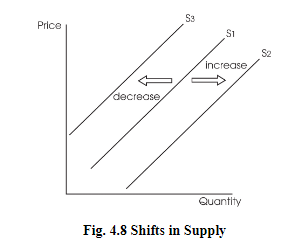
The change occurs along the supply curve.
Shift in supply is due to the determinants of supply.
Determinants of supply are the factors that influence the supplier to offer more or fewer goods at the same price.
Determinants of Supply
The ROTTEN Acronym:
R = Resources
The cost of production (land, labor, capital) has an inverse impact on the supply.
When the cost of these increases, the supplier decides to produce less of the products since he is unable to afford the production cost.
O = Other good prices
Suppliers who produce more than one product (profit-maximizing firms) have an easier time switching to the production of another product if issues do a rise in prices.
T = Taxes
Taxes are added up to the unit cost of production, thus making it more expensive.
T = Technology
Newer technology causes the cost of production to decline and helps improve the efficiency of the supplier.
E = Expectations of the supplier
If suppliers expect prices to increase in the future, they will hold back supply for the current time with the future goal of earning more profit later (and vice versa).
N = Number of competitors
As the number of sellers increases in the market, the supply automatically increases.
This allows consumers more choices at a lower price due to an increase in competition.
Summing up:
Supply increases:
R = increase
O = decrease
T = decrease (taxes)
T = increase (technology)
E = increase
N = decrease
Supply decreases:
R = decrease
O = increase
T = increase (taxes)
T = decrease (technology)
E = decrease
N = increase
1.6 Market Equilibrium
Market Equilibrium
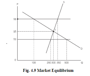
The market equilibrium price is that price that the market sets, where buyers buy the exact amount which the sellers are willing to produce.
It’s also known as market-clearing price.
Market Disequilibrium
This occurs when there is a shortage or surplus in the market.
Consider the price of $8 where the demand is 100 and the corresponding supply is 350.
This surplus is what creates market disequilibrium.
Changes in Equilibrium (solving demand and supply-related questions)
Is it supply, demand, or both?
Is it an increase (shift to the right) or a decrease (shift to the left)?
Supply increases towards the right and decreases towards the left.
Demand increases towards the right (moves upwards) and decreases towards the left (moves downwards).
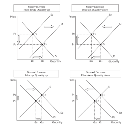
When supply is constant and only demand increases, equilibrium price, and quantity increase.
When supply is constant and only demand decreases, equilibrium price and quantity decrease.
When demand is constant and only supply increases, equilibrium price, and quantity decrease.
When demand is constant and only supply decreases, equilibrium price and quantity increase.
Key concepts:
Market shortage: shortage (Excess demand) - Also known as excess demand, a shortage exists at a market price when the quantity demanded exceeds the quantity supplied. The price rises to eliminate a shortage.
Market surplus: Surplus (Excess supply) - Also known as excess supply, a surplus exists at a market price when the quantity supplied exceeds the quantity demanded. The price falls to eliminate a surplus.
Changes in equilibrium:
Increase in demand:
eq (price) = increases
eq (quantity) = increases
Decrease in demand:
eq (price) = decreases
eq (quantity) = decreases
Increase in supply:
eq (price) = decreases
eq (quantity) = increases
Decrease in supply:
eq (price) = increases
eq (quantity) = decreases