Macroeconomics
AP Macroeconomics
Unit 5: Long-Run Consequences of Stabilization Policies
Gourishankar Residential English Medium School
fiscal and monetary policy
Phillips curve
shifting SRAS
The long-run Phillips curve
money growth
inflation
cost-push inflation
demand-pull inflation
wage-price spiral
theory of monetary neutrality
quantity theory of money
deficits and the national debt
surplus
state and local debts
crowding out
long run impact
economic growth
productivity
public policy
supply-side policies
saving and investment

Unit 5: Long-Run Consequences of Stabilization Policies
5.1 Fiscal and Monetary Policy Actions in the Short-Run
Fiscal Policy
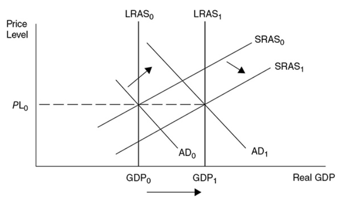
Classical Adjustment from Short-Run to Long-Run Equilibrium
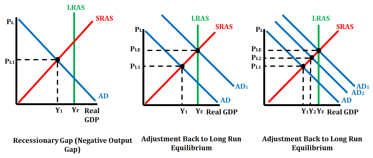
Adjustment to a recessionary gap:
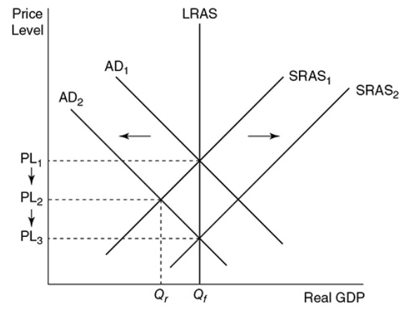
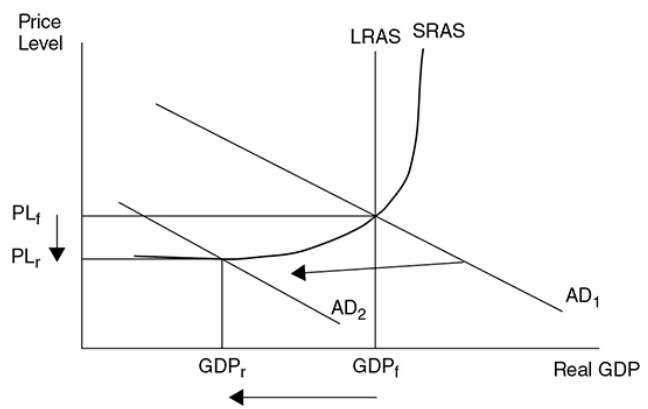
Based on this graph, the economy is currently operating at full employment. If consumers and firms begin to lose confidence in the labor market and overall economy, AD shifts to the left.
In the short run, this causes a recessionary gap as real GDP falls to GDPr meaning that unemployment rises and aggregate price levels fall from PL1 to PL2.
NOTE - One of the hallmarks of a recession is a decreased demand for many factors of production.
This recessionary gap fixes itself since the prices of the products will decrease, causing a gradual rightward shift of the SRAS curve to SRAS2. The curve shifts to the right until the gap is closed and the economy is back at GDPf.
Adjustment to an inflationary gap:

When the AD curve increases, an inflationary gap happens to cause an increase in real GDP to GDPi (lower unemployment rate) and an increase in the aggregate price level to PL2.
When this happens, there’s stronger demand for labor and all of the other factors of production causing factor prices to rise. As the factor prices rise, the SRAS curve shifts to the left to SRAS2 eventually eliminating the inflationary gap, but at a higher aggregate price level of PL3.
Monetary Policy
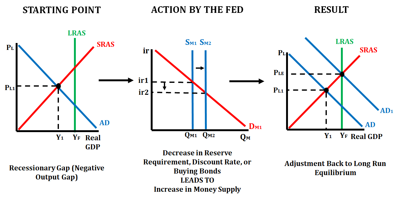
Recessionary Gap Correction
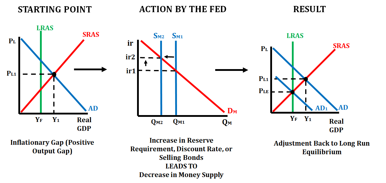
Inflationary Gap Correction
Coordination of Fiscal and Monetary Policy
The central bank develops monetary policy and is independent of Congress and the president. This is a critical balance to fiscal policy that can be heavily politicized.
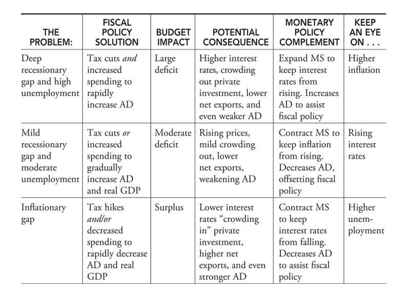
In a deep recessionary gap, expansionary monetary policy could be used to assist expansionary fiscal policy in quickly moving to full employment. The risk then becomes a burst of inflation.
In a mild recessionary gap, contractionary monetary policy could be used to offset expansionary fiscal policy to gradually move to full employment. The risk then becomes rising interest rates.
In an inflationary gap, contractionary monetary policy could be used to assist contractionary fiscal policy to put downward pressure on the price level. The risk then becomes a rising unemployment rate.
5.2 Phillips Curve
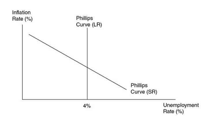
Phillips curve - A graphical device that shows the relationship between inflation and the unemployment rate. In the short run, it’s downward sloping, and in the long run, it’s vertical at the natural rate of unemployment.
It shows the inverse relationship between inflation and the unemployment rate.
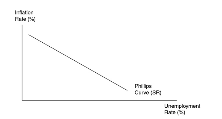
The possibility of deflation at extremely high unemployment rates means that the Philips curve may continue to fall below the x-axis.
Shifts in AD
Demand-pull inflation - This inflation is the result of stronger consumption from all sectors of AD as it continues to increase in the upward-sloping range of SRAS.
If AD increases from AD0 to AD1 in the nearly horizontal range of SRAS, the price level may only slightly increase, while real GDP significantly increases and the unemployment rate falls.
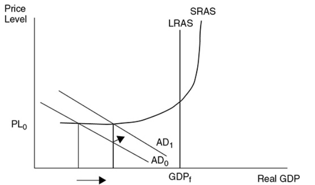
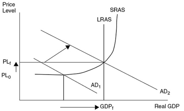
If AD continues to increase to AD2 in the upward-sloping range of SRAS, the price level begins to rise and inflation is felt in the economy.
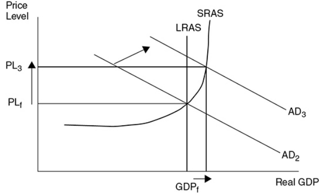
If AD increases much beyond full employment to AD3, inflation is quite significant and real GDP experiences minimal increases.
Recession - In the AD and AS models, a recession is typically described as falling AD with a constant SRAS curve. Real GDP falls far below full employment levels and the unemployment rate rises.
Deflation - A sustained falling price level, usually due to severely weakened aggregate demand and a constant SRAS.
If aggregate demand weakens, the opposite is expected. One of the most common causes of recession is falling AD since it lowers real GDP and increase the s unemployment rate. Deflation is expected here.
Shifting SRAS
Supply-side boom - When the SRAS curve shifts outward and the AD curve stays constant, the price level falls, real GDP increases and the unemployment rate falls.
The simplified
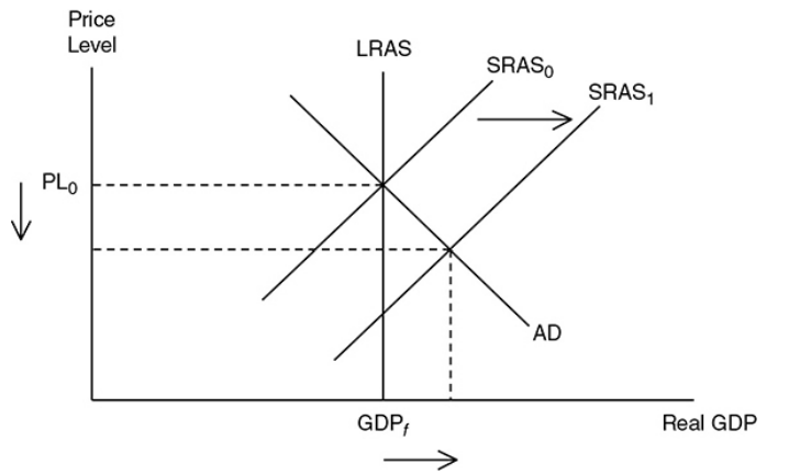
If nominal input prices fall, the SRAS curve shifts to the right.
Stagflation (Cost-push inflation) - A situation in the macroeconomy when inflation and the unemployment rate are both increasing. This is most likely the cause of falling SRAS while AD stays constant.
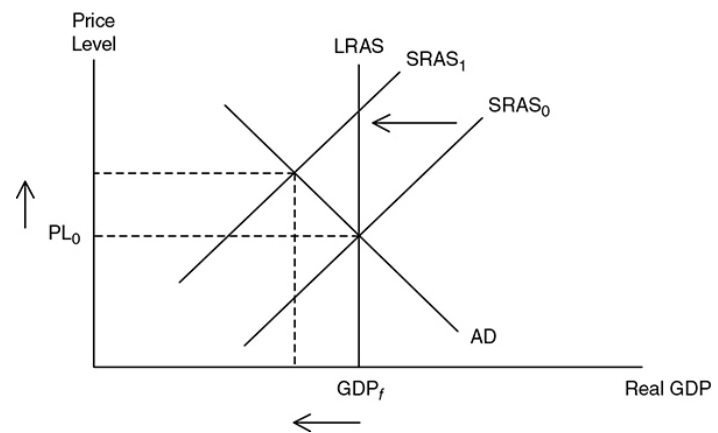
An increase in SRAS is the best possible macroeconomic situation. A decrease is one of the worst.
A decrease creates inflation, lowers real GDP, and increases the unemployment rate.
The Long-Run Phillips Curve
The AS model assumes that the long-run AS curve is vertical and at full employment. This causes the Philips curve to be vertical at the natural rate of employment.
5.3 Money Growth and Inflation
Inflation
It is the result of increasing the money supply.
It closes the recessionary gap.
In deflation:
The money supply decreases.
The inflationary gap will be closed.
Price level will increase.
Demand-Pull Inflation
It is caused by an increase in consumer demand.
It happens when AD shifts to the right with consumers spending more.
The price level increases.
Real GDP increases.
It is caused by too much government deficit spending.
It usually drives up AD.
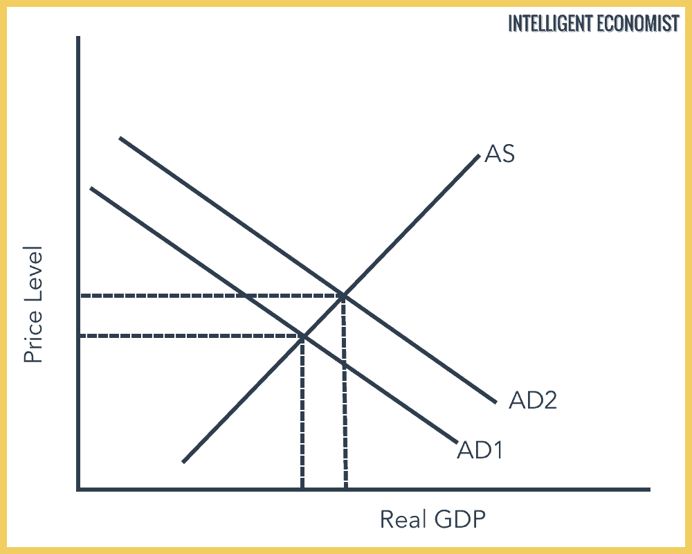
Seen in the graph above, AD1 shifts to the right to AD2, increasing both price and real GDP. This is also known as the inflationary gap, and it is corrected through long-run adjustment and contractionary fiscal or monetary policies.
Cost-Push Inflation
It is caused when production is decreased.
Anything which disturbs production and decreases supply is to be cost-push inflation.
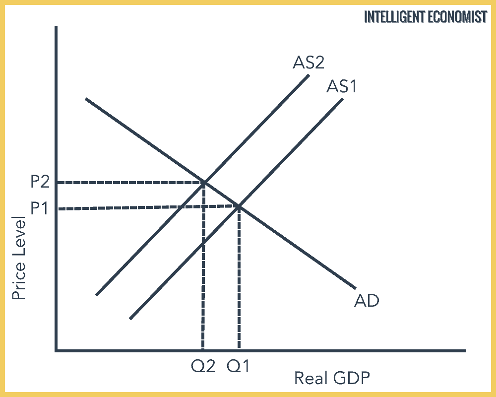
With this type of inflation, supply shortages happen, leading to AS1 (short-run in this case) shifting to the left to AS2. This drives the price level to increase but the real GDP to decrease. This is a bad example of inflation because it's a little harder to fix.
Wage-Price Spiral
A self-perpetuating spiral where demand rises and supply goes down.
Demand-pull and Cost-push are working together, which is the worst case with inflation.
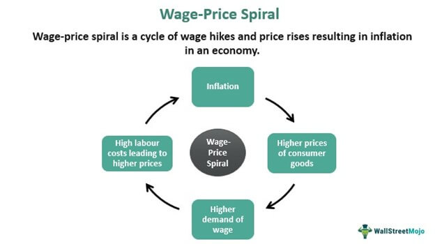
Everything is now at higher prices, which will lead to more inflation, then higher prices of everything, then higher demand for wages, then higher production costs, and it keeps going on.
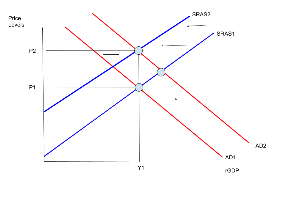
As seen in the graph, we have a double shifter. AD is shifting to the right, while SRAS is shifting to the left. As a result, real GDP is unchanged, but we still have an increase in the price level.
Inflation due to Changes in the Money Supply
Inflation can happen due to changes in monetary supply.
Every time they increase or decrease the money supply, the price level can be indirectly affected.
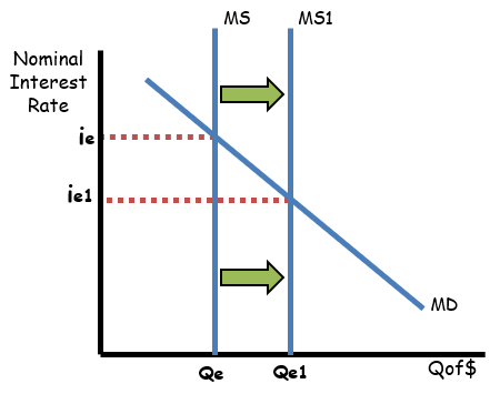
MS, meaning money supply, was increased by the Fed. Consequently, the interest rate and quantity of money increased. This indirectly leads to an increase in price, thus inflation.
Theory of Monetary Neutrality
A change in the money supply does not affect the economy.
Only the dollar values are changed and nothing else.
The theory of monetary neutrality is a nice way of saying money doesn’t matter.
Quantity Theory of Money
The critical link between monetary policy and real GDP is the relationship between changes in money supply, the real interest rate, and the level of private investment.
If the money supply increases and there is no increase in investment, expansionary monetary policy would have no effect on real GDP.
The quantity theory of money - A theory that asserts that the quantity of money determines the price level and that the growth rate of money determines the rate of inflation.
It predicts that any increase in the money supply only causes an increase in the price level.
Equation of exchange - A way to view the quantity theory of money. The equation says that nominal GDP (P × Q) is equal to the quantity of money (M) multiplied by the number of times each dollar is spent in a year (V). MV = PQ.
The velocity of money - The average number of times that a dollar is spent in a year. V = PQ/M.
Ex. → If in a given year the money supply is $100 and nominal GDP is $1,000, each dollar must be spent 10 times; V = 10.
If the money supply (M) increases, the increase must be reflected in the other variables. To accommodate an increase, the velocity of money must fall, the price level must rise, or the economy’s output of goods and services must increase.
Economists believe that the quantity of output produced in a given year is a function of technology and the supply of resources. Therefore, the increased money supply is going to only create inflation.
5.4 Deficits and the National Debt
Key Vocabulary
Fiscal Stimulus—The use of expansionary fiscal policy, including an increase in government spending, a decrease in personal taxes, or an increase in income transfers.
Fiscal Restraint—The use of contractionary fiscal policy, including a decrease in government spending, an increase in personal taxes, or a decrease in income transfers.
Government Revenue—The total income gained by the government at all levels, through tax policies, including income taxes, excise taxes, and regulatory taxes.
Government Expenditures—The total spending payments made by the government at all levels, including discretionary and non-discretionary purchases.
Budget Surplus—The condition that exists when government revenues exceed government expenditures. This occurs when tax revenues are more than government purchases plus transfer payments in a given year.
Budget Deficit—The condition that exists when government expenditures exceed government revenues. This occurs when tax revenues are less than government purchases plus transfer payments in a given year.
National Debt—The accumulation of deficits over multiple years.
US National Debt
The US government’s debt is immense.
As of 2023, the debt is a huge $31 trillion!
Surplus and Deficit
Surplus happens when the difference between tax revenues and government spending is positive.
Deficit happens when the government spends more than its received revenue.
The US government has three areas to spend a certain amount of money every year called mandatory spending.
Social Security
Medicare
Interest on the national debt
State and Local Debts
The US is operating in a recessionary gap, where tax revenues are low and spending is high, leading to a deficit.
The US is operating in an expansionary gap, where tax revenues are high and spending low, leading to a surplus.
In both scenarios, if the Constitution required the state government to balance the budget to exactly zero here's what would happen:
Government implements higher taxes and less spending, but this is a recipe for a recession!
Government implements lower taxes and more spending, but this is a recipe for inflation!
5.5 Crowding Out
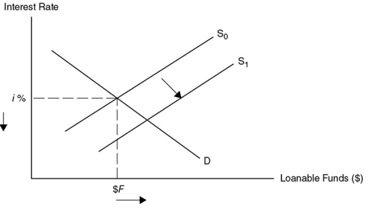
Crowding out effect - It is the economic theory that public sector spending can lessen or eliminate private sector spending.
The government’s budget deficit increases demand for loanable funds, but it reduces the number of available loan funds for private investors.
Less investment happening by the private sector means national economic growth is not happening.
This reduces demand and brings the economy back to where it started: a recessionary gap.
Federal Government is the largest demander for loanable funds.
The graph on left shows an economy in a recessionary gap.
The graph in middle shows the rightward shift of aggregate demand.
It can correct a recessionary gap when the government increases its spending.
The graph on the right shows what can happen when crowding out occurs.
Instead of government spending correcting the economy, they choose to spend money on a good or service that will decrease or eliminate private spending, causing the economy to move only from AD to AD2. When crowding out occurs, the economy does not quite get back to long-run equilibrium.
Long-Run Impact
Crowding out is not always an issue.
Sometimes, there will be enough loanable funds for everyone.
The government borrows loanable funds but siit its is already in deficit the situation just worsens and turns into a looming depression.
Economy:
Crowding out prolongs -
economic growth reduced.
economy might start going downhill
widen the recessionary gap.
finally results in economic doom.
Infrastructure:
Crowding out prolongs -
private investments decrease.
low investments leads to a decrease in inefficiency in building things.
5.6 Economic Growth
GDP per capita
Growth is measured through real GDP per capita.
GDP per capita = real GDP / population
If GDP per capita increases, economy grew.
Aggregate Production Function
The aggregate production function is a function that shows the relationship between production and capital.
It shows long-run economic growth.
Production Possibilities
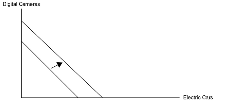
This graph shows that the country’s production possibilities in electric cars and digital cameras grows over time if
The quantity of economic resources increases,
The quality of those resources improves.
The nation’s technology improves.
Productivity
Productivity - The quantity of output that can be produced per worker in a given amount of time.
If the labor force of a country produces more output per worker from one year to the next, productivity has increased and the PCC shifted outwards.
Determinants of Productivity
All of these require an investment, funds that come from savings. Firms invest in physical capital and individuals invest in human capital. Countries invest in natural resources entrepreneurs invest in technology.
Stock of physical capital - When the quantity of physical capital in an economy is increased, in many cases, the capital helps increase the quantity of more capital.
Human capital - The amount of knowledge and skills that labor can apply to the work that they do and the general level of health that the labor force enjoys.
Natural resources - Productive resources provided by nature.
Nonrenewable resources - Natural resources that cannot replenish themselves. Coal is a good example.
Renewable resources - Natural resources that can replenish themselves if they are not overharvested. Lobster is a good example.
Technology - A nation’s knowledge of how to produce goods in the best possible way.
5.7 Public Policy and Economic Growth
Public Policy
Types of Public Policy:
Increase in education spending
By increasing investment in the education of workers, those workers are more effective and can produce more. Improving human capital increases the quality of labor available, which causes an increase in economic growth.
Increase in infrastructure spending
For example, if the government sets up dependable transportation systems, then they are helping businesses get inputs to production, and get goods to customers. This means that government spending on infrastructure raises government spending and contributes to the growth of real GDP in the long run.
Policies that spur innovation
By creating policies that promote innovation, the government can promote economic growth in the long run. For example, the government can create policies that protect intellectual property (patents), which would give private companies a greater incentive to create that intellectual property. By promoting creativity and entrepreneurship, we will be able to increase real GDP in the long run.
Increasing employment
By increasing employment, more workers will lead to increased productivity, thus leading to economic growth.
Supply-Side Policies
Supply-side fiscal policy - Fiscal policy centered on tax reductions targeted to AS so that real GDP increases with very little inflation.
The main justification is that lower taxes on individuals and firms increase incentives to work, save, invest, and take risks.
Saving and Investment
Investment tax credit - A reduction in taxes for firms that invest in new capital like a factory or piece of equipment.
Lower income taxes create disposable income for households, increasing both consumption and savings from households and the profitability of investment for firms. This allows for an increase in the productive capacity of the country because more capital stock is accumulated. As well, this increases the long-run AS curve. Tax incentives to increase savings and investment are likely to increase AD.
How lower taxes can increase AS and AD
Productivity incentives - Lower taxes mean workers take more of their pay home, which might prompt wage earners to work harder, take less time off, and be more productive.
Risk-taking - Lowering the tax rate on profits increases the expected rate of return and encourages more investment.