


Chapter 8: Probability and Random Variables
In this chapter, we’ll learn about the basic rules of probability, what it means for events to be independent, and about discrete and continuous random variables, simulation, and rules for combining random variables.
Probability
The probability of an event is the predicted long-run relative frequency of occurrences of that event.
If we repeat a random process many times, the predicted proportion of outcomes that are “successes” is the probability of success.
The probability of an event must be between 0 and 1.
A probability of 0 means the event is impossible.
A probability of 1 means the event is certain.
Example:
If we roll a six-sided die, we know that we will get a 1, 2, 3, 4, 5, or 6, but we don’t know which one of these we will get on the next trial. What are two ways we could estimate the probability of rolling a 6?
Solution:
We could estimate the probability experimentally by rolling a die 300 times. The results of one such set of rolls are shown below.
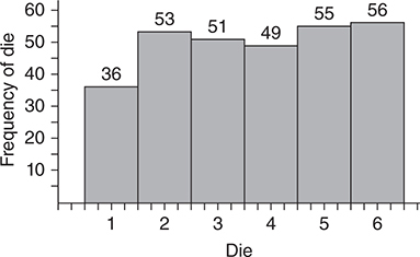
Out of 300 trials, 56 were successes.
Thus, probability = 56/300 = 0.187
We could also estimate the probability theoretically by assuming each possible result is equally likely.
If that is the case, then the probability of each number appearing = 1/6 = 0.167
Outcome:
One of the possible results of a chance process.
Generally we refer to the most basic kind of occurrences as outcomes.
Event:
A collection of outcomes or simple events.
Example:
The possible outcomes for the roll of a single die are 1, 2, 3, 4, 5, and 6.
Rolling an even number would be an event that consists of the outcomes 2, 4, and 6.
Sample Spaces and Events
A sample space is a complete list of disjoint outcomes or events.
“Complete” means that you have all the possibilities listed.
“Disjoint” means that the events have no outcomes in common.
Only one event can happen in a particular trial.
Example:
Consider the experiment of flipping two coins. Sample space is HH, HT, TH, TT. The list is complete because there is no other possibility for tossing two coins. The list is disjoint because a pair of coin tosses can result in only one of those outcomes.
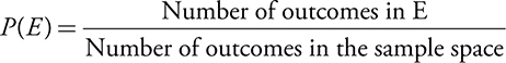
If we let E = the event of interest, then the probability of E, written P(E) is given by:
The sum of the probabilities of all possible outcomes in a sample space is 1.
Example 1:
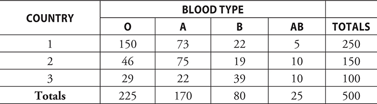
The table below represents country of origin and blood type for 500 people attending a large conference.
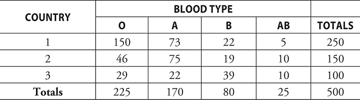
If we were to randomly select one person from this population of people attending the conference, how would you verify that the outcomes in the table define a sample space?
Solution:
You could check that each person falls into exactly one category in the table.
For this, check that the row and column totals are actually the sum of the numbers in the cells.
If they are not, it would mean that either some people fall into more than one category or there would be people not included in the table.
In this table, the totals are actually the sum of the numbers in the cell. This means the list is disjoint and complete.
Example 2:
Using the data above, if you randomly select a person from the population of people attending the conference, what is the probability the person has blood type A?
Solution:
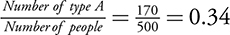
There is a 34% probability that a randomly selected person attending this conference has blood type A.
The numbers in the total row and the total column are called marginal frequencies,
The cells in the middle of the table give the joint frequencies.
Dividing a frequency in a cell by the total gives the proportion of cases in that cell.
This is also called the relative frequency.
If you look at randomly selecting an individual from the population, those relative frequencies give the probability of selecting a person from that cell.
Probabilities of Combined Events
P (A or B):
The probability that either event A or event B occurs (or both).
Using set notation, P (A or B) can be written P(A ∪ B) spoken as “A union B”.
P (A and B):
The probability that both event A and event B occur.
Using set notation, P (A and B) can be written
P(A ∩ B) spoken as “A intersect B.”
Addition Rule:
P (A or B) = P (A) + P (B) – P(A and B)
Example:
If you randomly select one person from the population from the table used previously, use the addition rule to find P(Type A or Country #2).
Solution:
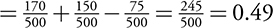
P(Type A or Country #2) = P (Type A) + P (Country #2) – P (Type A and Country #2)
Complement of an event A:
Events in the sample space that are not in event A.
The complement of an event A is symbolized by Ā , or A^c.
Furthermore, P(Ā) = 1 − P (A).
Example:
If you randomly select a person attending this conference, what is the probability that the person has blood type A, O, or AB?
Solution:
You could simply subtract the marginal probability for the one remaining category, Type B, and subtract that from 1.
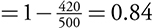
P (A, O, or AB) = 1 − P (Type B)
Conditional Probability
The probability of A given B
Assumes we have knowledge of an event B having occurred before we compute the probability of event A.
This is symbolized by P (A | B).
Example (Conditional Probability from a table):
If you randomly select a person with blood type A, what is the probability that this person is from Country 3?
Solution:
You know the person has blood type A. We need to look only at the relevant column.
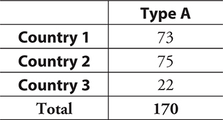
P (Country 3 | Type A) = 22/170 = 0.129
Example (Conditional Probability from a tree):
Suppose a computer company has manufacturing plants in three states. Fifty percent of its computers are manufactured in California, and 85% of these are desktops; 30% of computers are manufactured in Washington, and 40% of these are laptops; and 20% of computers are manufactured in Oregon, and 40% of these are desktops. All computers are first shipped to a distribution site before being sent to stores.
a)If you picked a computer at random from the distribution center, what is the probability that it is a laptop?
b) What are the chances that if you randomly selected a laptop from the distribution center, it is a laptop that was manufactured in California?
Solution:
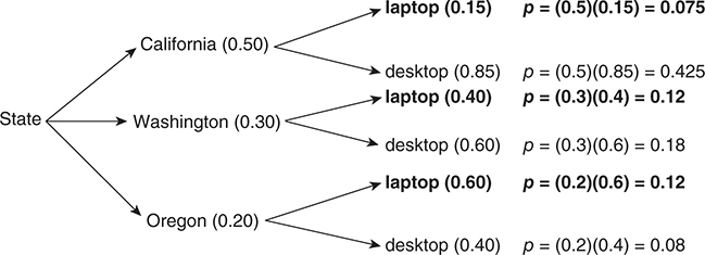
a) Sum of all probabilities = 1
Now, P (laptop) = 0.075 + 0.12 + 0.12 = 0.315.
b) P (California | laptop) = 0.075/0.315) = 0.238.
Independent Events
A and B are independent if the probability of A, given that B occurred, is the same as the probability that A occurred and vice versa.
In symbols, A and B are independent if and only if P (A|B) = P (A) or P (B|A) = P (B).
Example:
Consider drawing one card from a standard deck of 52 playing cards.
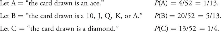
i)Are A and B independent?
ii)Are A and C independent?
Solution:
i) P (A|B) =
P (the card drawn is an ace | the card is a 10, J, Q, K, or A)
= 4/20
= 1/5.
Since P (A) = 1/13, knowledge of B has changed what we know about A.
In this case, P (A) ≠ P (A|B), so events A and B are not independent.
ii) P (A|C) =
P (the card drawn is an ace | the card drawn is a diamond)
= 1/13
In this case, P (A) = P (A | C) so that the events “the card drawn is an ace” and “the card drawn is a diamond” are independent.
The Multiplication Rule:
P (A and B) = P (A) . P (B|A)
If events A and B are independent,
P (B|A) = P(B)
so P (A and B) = P (A). P (B)
Example:
A and B are two mutually exclusive events for which P (A) = 0.3 and P (B) = 0.25. Find P (A or B). Solution: P (A or B) = 0.3 + 0.25 = 0.55.
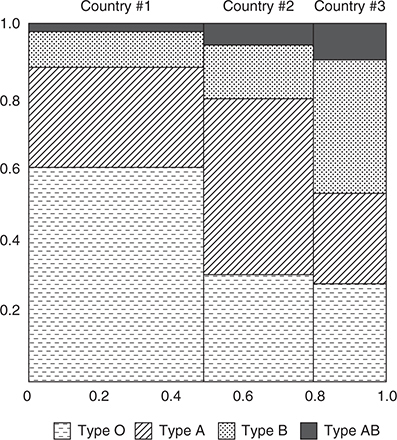
Segmented Bar Graphs and Mosaic Plots
A segmented bar graph takes bars of equal length and equal width for each of the groups and divides them up into segments that represent the percentage for each of the categories.
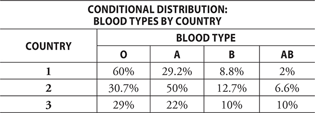
We use conditional relative frequencies
Looking at the previously used table:
To find relative frequencies, we take each country as its own group and calculate based on that condition.
For example, there are 150 people out of 250 in Country 1 with blood type O, and this would be a conditional relative frequency of 0.60 or 60%.
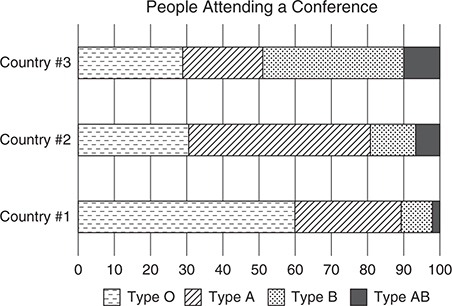
Question: Based on this segmented bar graph, do you believe that blood type and country are independent?
Answer: Since the segments are so differently sized in each bar, it does not appear that blood type and country are independent.
Another type of plot that can be used with these data is a mosaic plot.
A mosaic plot helps preserve the relative sizes of the groups by keeping the heights the same but making the widths of the bars proportional to the group size.
Random Variables:
A random variable , X , is a numerical value assigned to an outcome of a random phenomenon.
Particular values of the random variable X are often given lowercase names, such as x to represent a general value or k to represent a specific value.
It is common to see expressions of the form P(X=x) or P(X=k).
Example:
If we roll a fair die, the random variable X could be the face-up value of the die. The possible values of X are {1, 2, 3, 4, 5, 6}. P ( X = 2) = 1/6.
Discrete Random Variables
A random variable with a countable number of outcomes.
It is a variable whose values are separated by gaps.
Example: The number of left-handed people in a sample of 100 people, for example, can only take on whole number values from 0 to 100.
Continuous Random Variables
A random variable that takes on values associated with one or more intervals on the number line.
The continuous random variable X can assume infinitely many outcomes within an interval.
Example: Heights of people, although the reported heights may be discrete if they are reported to the nearest inch.
Probability Distribution of a Random Variable
The possible values of the random variable X together with the probabilities corresponding to those values.
Example:
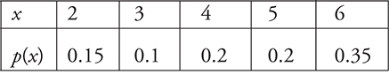
Let X be the number of boys in a three-child family. Assuming that the probability of a boy on any one birth is 0.5, the probability distribution for X is
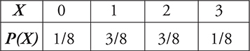
The probabilities Pi of a DRV satisfy two conditions:
0 ≤ Pi ≤ 1 or Every probability is between 0 and 1.
ΣPi = 1 or the sum of all probabilities is 1.
Some Formulae:
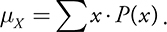
The mean of a discrete random variable, also called the expected value , is given by
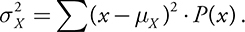
The variance of a discrete random variable is given by
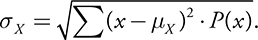
The standard deviation of a discrete random variable is given by
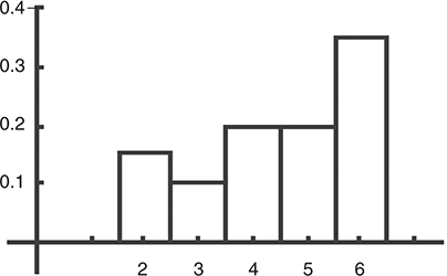
Probability Histogram
The following is a TI-83/84 probability histogram for discrete variables of the probability distribution we used in a couple of the earlier examples.
For a probability Distribution for a Continuous Random Variable, Here are a few things to remember:
The probability of any individual value is 0. That is, if a is a point on the horizontal axis, P(X=a)=0.
To find the probability of an event, you must find the probability that x falls in some given interval. To do this, use the normalcdf function on your calculator.
Normal Probabilities:
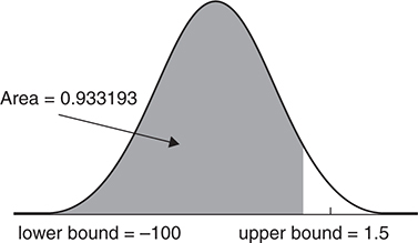
Example:
In a standard normal distribution, what is the probability that z < 1.5?
Solution:
The standard normal table gives areas to the left of a specified z -score. From the table, we determine that the area to the left of z = 1.5 is 0.9332.
Simulation and Random Number Generation
A simulation utilizes some random process to conduct numerous trials of the situation and then counts the number of successful outcomes to arrive at an estimated probability.
The more trials, the more confidence we can have that the relative frequency of successes accurately approximates the desired probability.
law of large numbers states that the proportion of successes in the simulation should become, over time, close to the true proportion in the population.
Example:
A coin is known to be biased in such a way that the probability of getting a head is 0.4. If the coin is flipped 50 times, how many heads would you expect to get?
Solution:
Let 0, 1, 2, 3 be a head and 4, 5, 6, 7, 8, 9 be a tail. If we look at 50 digits beginning with the first row, we see that there are 18 heads, so the proportion of heads is 18/50 = 0.36. This is close to the expected value of 0.4.
Sometimes the simulation will be a wait-time simulation . In the example above, we could have asked how long it would take, on average, until we get five heads.
Transforming and Combining Random Variables
If X is a random variable, we can transform the data by adding a constant to each value of X , multiplying each value by a constant, or some linear combination of the two.
For example, if values in our dataset ranged from 8500 to 9000, we could subtract, say, 8500 from each value to get a dataset that ranged from 0 to 500.
Rules for the Mean and Standard Deviation of Combined Random Variables
Example:
One contractor can finish a particular job, on average, in 40 hours ( μx = 40). Another contractor can finish a similar job in 35 hours ( μy = 35). If they work on two separate jobs, how many hours, on average, will they bill for completing both jobs?
Solution:
It should be clear that the average of X + Y is just the average for X plus the average for Y. That is, μX ± Y = μX ± μY .
To combine the variances, we use:
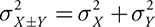
To combine standard deviations,
Example:
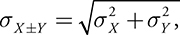
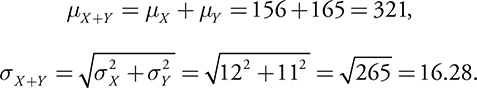
A private school offers an admission test on the first Saturday of November and the first Saturday of December each year. In 2008, the mean score for hopeful students taking the test in November was 156 with a standard deviation of 12. For those taking the test in December, the mean score was 165 with a standard deviation of 11. What are the mean and the standard deviation of the total score X + Y of all students who took the test in 2008?
Solution:
It is reasonable to assume that X and Y are independent. Therefore:
Click the link to go to the next chapter: