The Law of Large Numbers

• Law of large numbers - states that when an experiment is performed a large number of times, the relative frequency of an event tends to become closer to the true probability of the event; that is, probability is long-run relative frequency. There is a sense of predictability about the long run.

The law of large numbers has two conditions:

• First, the chance event under consideration does not change from trial to trial.

• Second, any conclusion must be based on a large (a very large!) number of observations.

➥ Example 4.1

There are two games involving flipping a fair coin. In the first game, you win a prize if you can throw between 45% and 55% heads. In the second game, you win if you can throw more than 60% heads. For each game, would you rather flip 20 times or 200 times?

Solution: The probability of throwing heads is 0.5. By the law of large numbers, the more times you throw the coin, the more the relative frequency tends to become closer to this probability. With fewer tosses, there is greater chance of wide swings in the relative frequency. Thus, in the first game, you would rather have 200 flips, whereas in the second game, you would rather have only 20 flips.

Basic Probability Rules

➥ Example 4.2

A standard literacy test consists of 100 multiple-choice questions, each with five possible answers. There is no penalty for guessing. A score of 60 is considered passing, and a score of 80 is considered superior. When an answer is completely unknown, test takers employ one of three strategies: guess, choose answer (c), or choose the longest answer. The table below summarizes the results of 1000 test takers.

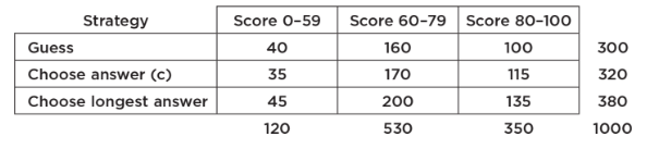
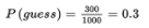
1. What is the probability that someone in this group uses the “guess” strategy?

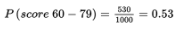
2. What is the probability that someone in this group scores 60–79?

3. What is the probability that someone in this group does not score 60–79?

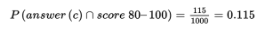
4. What is the probability that someone in this group chooses strategy “answer (c)” and scores 80–100 (sometimes called the joint probability of the two events)?

5. What is the probability that someone in this group chooses strategy “longest answer” or scores 0–59?

6. What is the probability that someone in this group chooses the strategy “guess” given that his or her score was 0–59?

7. What is the probability that someone in this group scored 80–100 given that the person chose strategy “longest answer”?

8. Are the strategy “guess” and scoring 0–59 independent events? That is, is whether a test taker used the strategy “guess” unaffected by whether the test taker scored 0–59?

9. Are the strategy “longest answer” and scoring 80–100 mutually exclusive events? That is, are these two events disjoint and cannot simultaneously occur?

Solution:

2. 

3. P(does not score 60–79) = 1 − P(score 60–79) = 1 − 0.53 = 0.47

4. 

5. 

6. 

7. 

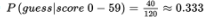
8. We must check if P (guess|score 0–59) = P(guess). From (f) and (a), we see that these probabilities are not equal (0.333 ≠ 0.3), so the strategy “guess” and scoring 0–59 are not independent events.

9. longest answer ∩ score 80–100 ≠ Ø and P(longest answer ∩ score 80–100)  = 135/1000 ≠ 0, so the strategy “longest answer” and scoring 80–100 are not mutually exclusive events.

Multistage Probability Calculations

➥ Example 4.3

On a university campus, 60%, 30%, and 10% of the computers use Windows, Apple, and Linux operating systems, respectively. A new virus affects 3% of the Windows, 2% of the Apple, and 1% of the Linux operating systems. What is the probability a computer on this campus has the virus?

Solution: In such problems, it is helpful to start with a tree diagram.

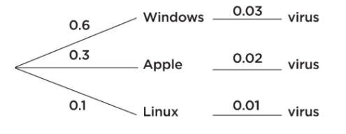
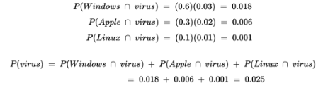
We then have:

Random Variables, Means (Expected Values), and Standard Deviations

• Often each outcome of an experiment has not only an associated probability but also an associated real number.

• If X represents the different numbers associated with the potential outcomes of some chance situation, we call X a random variable.

➥ Example 4.4

A charity holds a lottery in which 10,000 tickets are sold at $1 each and with a prize of $7500 for one winner. What is the average result for each ticket holder?

Solution: The actual winning payoff is $7499 because the winner paid $1 for a ticket. Letting X be the payoff random variable, we have:

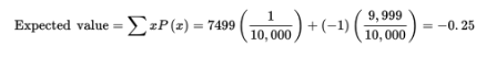
Thus, the average result for each ticket holder is a $0.25 loss. [Alternatively, we can say that the expected payoff to the charity is $0.25 for each ticket sold.]

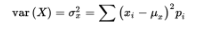
The mean of this new discrete random variable is ∑(xi − µx)2pi, which is precisely how we define the variance, σ2, of a discrete random variable:

➥ Example 4.5

A highway engineer knows that the workers can lay 5 miles of highway on a clear day, 2 miles on a rainy day, and only 1 mile on a snowy day. Suppose the probabilities are as follows:

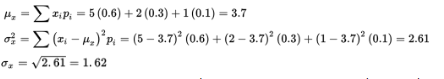
1. What are the mean (expected value), standard deviation, and variance?

2. Would it be surprising if the workers laid 10 miles of highway one day?

Solution:

In the long run, the workers will lay an average of 3.7 miles of highway per day. The number of miles the workers lay on a randomly selected day will generally vary about 1.62 from the mean of 3.7 miles.

2. 10 is 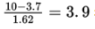standard deviations above the mean, so this would be very surprising!

Means and Variances for Sums and Differences of Sets

• When the random variables are independent, there is an easy calculation for finding both the mean and standard deviation of the sum (and difference) of the two random variables.

➥ Example 4.6

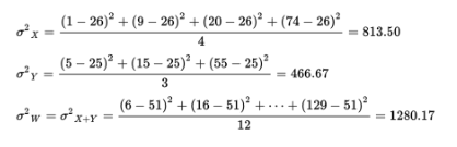
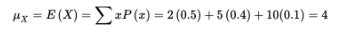
A casino offers couples at the hotel free chips by allowing each person to reach into a bag and pull out a card stating the number of free chips. One person’s bag has a set of four cards with X = {1, 9, 20, 74}; the other person’s bag has a set of three cards with Y = {5, 15, 55}. Note that the mean of set X is

1. What is the average amount a couple should be able to pool together?

Solution: Form the set W of sums: W = {1 + 5, 1 + 15, 1 + 55, 9 + 5, 9 + 15, 9 + 55, 20 + 5, 20 + 15, 20 + 55, 74 + 5, 74 + 15, 74 + 55} = {6, 16, 56, 14, 24, 64, 25, 35, 75, 79, 89, 129} and

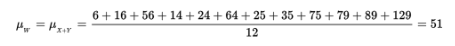
Finally, µW = µX + Y = µX + µY = 26 + 25 = 51. On average, a couple should be able to pool together 51 free chips.

2. How is the variance of W related to the variances of the original sets?

We can also calculate the standard deviation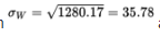

and conclude that the average pooled number of chips received by a couple is 51 with a standard deviation of 35.78.

Means and Variances for Sums and Differences of Random Variables

• The mean of the sum (or difference) of two random variables is equal to the sum (or difference) of the individual means.

• If two random variables are independent, the variance of the sum (or difference) of the two random variables is equal to the sum of the two individual variances.

➥ Example 4.7

An insurance salesperson estimates the numbers of new auto and home insurance policies she sells per day as follows:

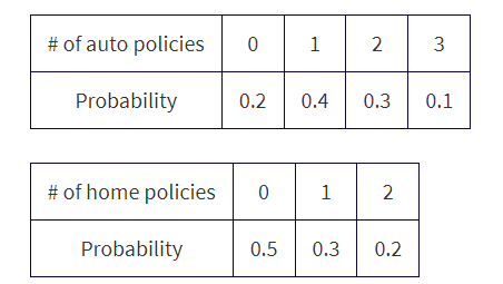
1. What is the expected value or mean for the overall number of policies sold per day?

2. Assuming the selling of new auto policies is independent of the selling of new home policies (which may not be true if some new customers buy both), what would be the standard deviation in the number of new policies sold per day?

Solution:

1. µauto= (0)(0.2) + (1)(0.4) + (2)(0.3) + (3)(0.1) = 1.3,
   µhome= (0)(0.5) + (1)(0.3) + (2)(0.2) = 0.7, and so
   µtotal = µauto + µhome = 1.3 + 0.7 = 2.0.

2. σ2auto= (0 − 1.3)2(0.2) + (1 − 1.3)2(0.4) + (2 − 1.3)2(0.3) + (3 − 1.3)2(0.1) = 0.81,
   σ2home = (0 − 0.7)2(0.5) + (1 − 0.7)2(0.3) + (2 − 0.7)2(0.2) = 0.61, and so, assuming independence, σ2total = σ2auto + σ2home = 0.81 + 0.61 = 1.42 and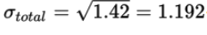

   

Transforming Random Variables

• Adding a constant to every value of a random variable will increase the mean by that constant.

• Differences between values remain the same, so measures of variability like the standard deviation will remain unchanged.

• Multiplying every value of a random variable by a constant will increase the mean by the same multiple. In this case, differences are also increased and the standard deviation will increase by the same multiple.

➥ Example 4.8

A carnival game of chance has payoffs of $2 with probability 0.5, of $5 with probability 0.4, and of $10 with probability 0.1. What should you be willing to pay to play the game? Calculate the mean and standard deviation for the winnings if you play this game.

Solution:

You should be willing to pay any amount less than or equal to $4.

What if $4 is added to each payoff?

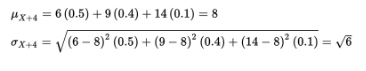
Note that µX+4 = µX + 4 and σX+4 = σX.

What if instead each payoff is tripled?

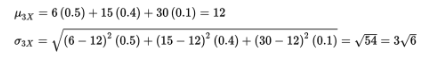
Note that µ3X = 3µX and σ3X = 3σX

Binomial Distribution

Probability distribution - is a list or formula that gives the probability of each outcome.

• For applications in which a two-outcome situation is repeated a certain number of times, where each repetition is independent of the other repetitions, and in which the probability of each of the two outcomes remains the same for each repetition, the resulting calculations involve what are known as binomial probabilities.

➥ Example 4.9

Suppose the probability that a lightbulb is defective is 0.1 (so probability of being good is 0.9).

1. What is the probability that four lightbulbs are all defective?

2. What is the probability that exactly two out of three lightbulbs are defective?

3. What is the probability that exactly three out of eight lightbulbs are defective?

Solution:

1. Because of independence (i.e., whether one lightbulb is defective is not influenced by whether any other lightbulb is defective), we can multiply individual probabilities of being defective to find the probability that all the bulbs are defective:

   (0.1)(0.1)(0.1)(0.1) = (0.1)4 = 0.0001

2. The probability that the first two bulbs are defective and the third is good is (0.1)(0.1)(0.9) = 0.009. The probability that the first bulb is good and the other two are defective is (0.9)(0.1)(0.1) = 0.009. Finally, the probability that the second bulb is good and the other two are defective is (0.1)(0.9)(0.1) = 0.009. Summing, we find that the probability that exactly two out of three bulbs are defective is 0.009 + 0.009 + 0.009 = 3(0.009) = 0.027.

3. The probability of any particular arrangement of three defective and five good bulbs is (0.1)3(0.9)5 = 0.00059049. We need to know the number of such arrangements.

   The answer is given by combinations:

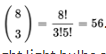
   Thus, the probability that exactly three out of eight light bulbs are defective is 56 × 0.00059049 = 0.03306744. [On the TI-84, binompdf(8,0.1,3)= 0.03306744.]

Geometric Distribution

• Suppose an experiment has two possible outcomes, called success and failure, with the probability of success equal to p and the probability of failure equal to q = 1 − p and the trials are independent. Then the probability that the first success is on trial number X = k is

  

➥ Example 4.10

Suppose only 12% of men in ancient Greece were honest. What is the probability that the first honest man Diogenes encounters will be the third man he meets? What is the probability that the first honest man he encounters will be no later than the fourth man he meets?

Solution:

This is a geometric distribution with p = 0.12. Then P(X=3) = (0.88)2(0.12) = 0.092928, where X is the number of men needed to be met in order to encounter an honest man. [Or we can calculate geometpdf (0.12, 3) = 0.092928.] This is a geometric distribution with p = 0.12. Then = geometcdf (0.12, 4) = 0.40030464. [Or we could calculate (0.12) + (0.88)(0.12) + (0.88)2(0.12) + (0.88)3(0.12) = 0.40030464.]

To receive full credit for geometric distribution probability calculations, students need to state:

1. Name of the distribution ("geometric" in the example above)

2. Parameter ("p = 0.12" in the example above)

3. The trial on which the first success occurs ("X = 3" in the first question above)

4. Correct probability (“0.092928” in the first question above)

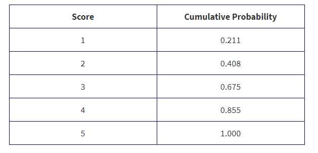
Cumulative Probability Distribution

• Probability distribution - is a function, table, or graph that links outcomes of a statistical experiment with its probability of occurrence.

• Cumulative probability distribution - is a function, table, or graph that links outcomes with the probability of less than or equal to that outcome occurring.

➥ Example 4.11

The scores received on the 2019 AP Statistics exam are illustrated in the following tables:

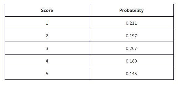
What is the probability that a student did not receive college credit (assuming you need a 3 or higher to receive college credit)?

Solution: the probability was 0.211 + 0.197 = 0.408 that a student received a 1 or 2 and thus did not receive college credit.