
Chapter 9: Inference: Testing Hypotheses
In this chapter, we form hypotheses and perform a test to determine whether we have convincing evidence that a particular hypothesis is incorrect.
Statistical Significance
First, we make an assumption about the population parameter.
This assumption is called the null hypothesis.
At the end of our analysis, if the result is so far from what we expected that we think something other than chance is operating, then the result is said to be statistically significant.
Example:
Todd claims that the average amount of money spent on ride tickets at a county fair is $50. If you have a random group of 50 fair goers and the average money spent on ride tickets for this group is $49.75, we have little reason to doubt Todd’s claim. But if the average for this group is $38, statisticians call this result statistically significant meaning that we would be unlikely to have a sample average this low if Todd’s claim is true.
P-Value
The P-value is what tells us just how unlikely a result actually is under the model based on the null hypothesis.
Example:
Suppose it turns out that the average amount of money a random group of 50 people spend on ride tickets at the county fair is $47.50. What is the probability of getting an observed mean this far below the expected $50 by chance alone if the true average is $50? Assume the population standard deviation is $8?
Is this finding significant at α = 0.05? At α = 0.01?
Solution:
Assume the population is normally distributed with mean = $50
standard deviation = $8.
The sampling distribution for this situation is pictured below:
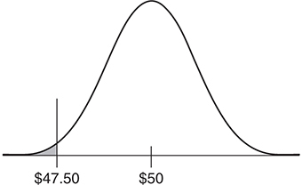
To find p value:
The p value thus comes out to be 0.014.
it’s the probability of getting a sample mean as far below $50 as we did by chance alone, assuming the model based on a mean of $50 is correct. This finding is significant at the 0.05 level but not at the 0.01 level.
Hypothesis Testing Procedure
In the hypothesis-testing procedure, a researcher does NOT look for evidence to support this hypothesis but instead looks for evidence against this hypothesis.
The process looks like this:
State the null and alternative hypotheses.
The null hypothesis is the one we are testing and usually states the claim is correct. Symbolized by H0.
The alternative hypothesis is the theory that the researcher wants to confirm by rejecting the null hypothesis. Symbolized by Ha.
There are three possible forms for the alternative hypothesis:

Identify which procedure you intend to use and show.
Compute the value of the test statistic and the P -value.
Give a conclusion, linked to your computations, in the context of the problem
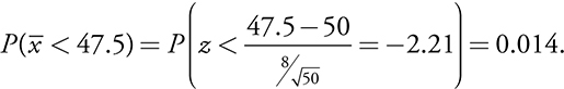
Inference for a Single Population Proportion
Example:
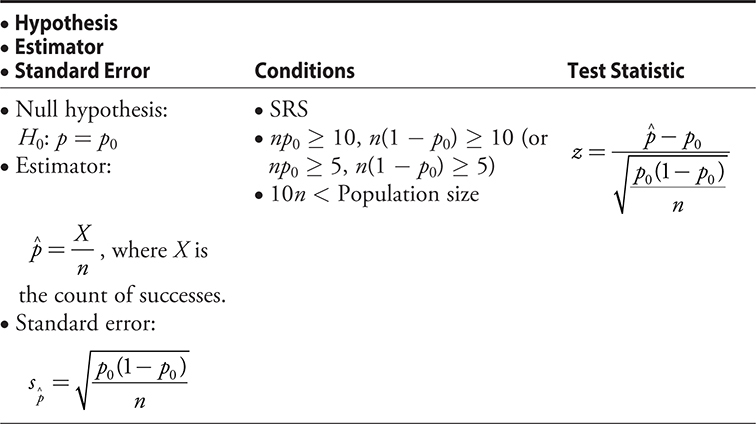
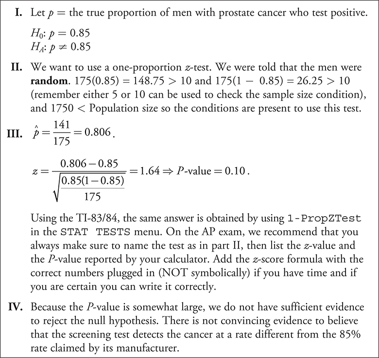
Consider a screening test for prostate cancer that its maker claims will detect the cancer in 85% of the men who actually have the disease. 175 random men who have been previously diagnosed with prostate cancer are given the screening test, and 141 of the men are identified as having the disease. Does this finding provide evidence that the screening test detects the cancer at a rate different from the 85% rate claimed by its manufacturer?
Solution:
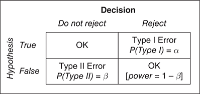
Type I and Type II Errors
If we are given a hypothesis, it may be true or it may be false. We can decide to reject the hypothesis or not to reject it. This leads to four possible outcomes:
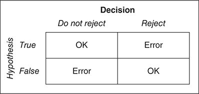
Type I Error: If the (null) hypothesis is true, and we mistakenly reject it. Denoted by alpha (α) which is the significance level.
Type II Error: If the hypothesis is false, and we mistakenly fail to reject it. Denoted by Beta(β).
The probability of correctly rejecting a false hypothesis is called the power of the test . The power of the test equals 1 − β.
Finally, then, our decision table looks like this:
Example:
Sticky Fingers is arrested for shoplifting. The judge, in her instructions to the jury, says that Sticky is innocent until proven guilty. That is, the jury’s hypothesis is that Sticky is innocent. Identify Type I and Type II errors in this situation and explain the consequence of each.
Solution:
Our hypothesis is that Sticky is innocent.
In Type I error Sticky is innocent, but because we reject innocence, he is found guilty.
The risk in a Type I error is that Sticky goes to jail for a crime he didn’t commit.
In type II error, Sticky goes free even though he is guilty.
To increase the power of a test:
Increase the sample size
Decrease the standard deviation of sample data.
Choose larger significance level (α)
Increase effect size. Effect size = (the difference between the hypothesized parameter and the true value)
z-Procedures versus t-Procedures
With proportions, we deal only with large samples—that is, with z -procedures.
When doing inference for a population mean, or for the difference between two population means, we typically use t -procedures because we do not know the population standard deviation.
t-Procedures are used when:
Sample is a simple random sample from the population.
The population from which the sample is drawn is normally distributed or sample size is large enough.
To check is the population is normally distributed, a stemplot, boxplot, dotplot, or normal probability plot can be used to show that there are no outliers or extreme skewness in the data itself.
Inference for a Single Population Mean
Use Test Statistic to identify the test to be used,
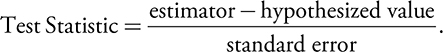
The estimator = x̄
The hypothesized value = µ0
In the null hypothesis H0 : µ = µ0
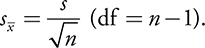
standard error =
Inference for the Difference Between Two Population Means
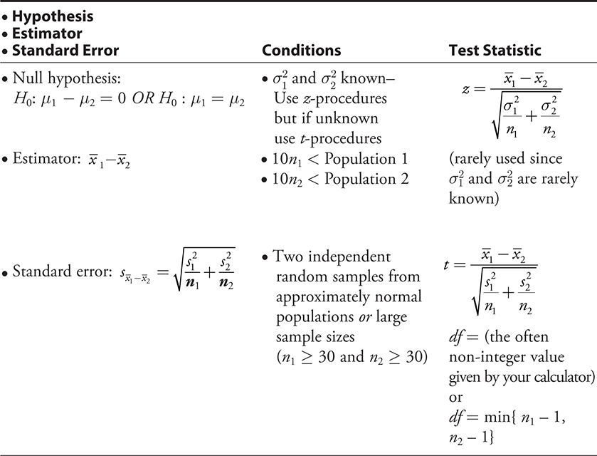
Matched Pairs
If samples in a 2 sample procedure are not drawn from independent populations—the data may be paired in some way.
In this case, run a one-sample hypothesis test on the differences.
Example:
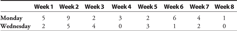
A company president believes that there are more absences on Monday than on other days of the week. The company has 45 workers. The following table gives the number of worker absences on Mondays and Wednesdays for a random sample of eight weeks from the past two years. Do the data provide evidence that there are more absences on Mondays?
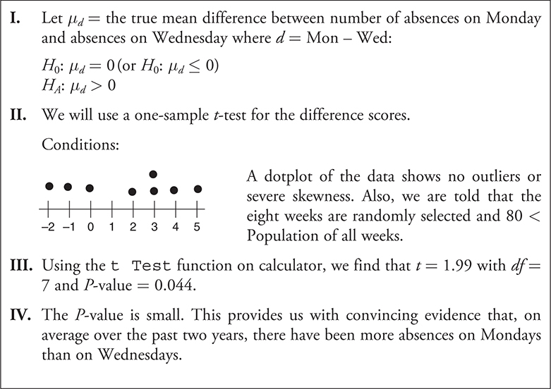
Solution:
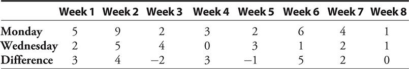
Because the data are paired on a weekly basis, the data we use for this problem are the differences between the days of the week for each of the eight weeks. Adding a row to the table that gives the differences.
Click the link to go to the next chapter