
AP Statistics Ultimate Guide
Unit 1: Exploring One-Variable Data
Categorical Variables
A categorical (or qualitative) variable takes on values that are category names or group labels.
The values can be organized into frequency tables or relative frequency tables or can be represented graphically by displays such as bar graphs (bar charts), dot plots, and pie charts.
➥ Example 1.1
During the first week of 2022, the results of a survey revealed that 1,100 parents wanted to keep the school year to the current 180 days, 300 wanted to shorten it to 160 days, 500 wanted to extend it to 200 days, and 100 expressed no opinion. (Noting that there were 2,000 parents surveyed, percentages can be calculated.)
A table showing frequencies and relative frequencies:
Desired School Length | Number of Parents (frequency) | Relative Frequency | Percent of Parents |
|---|---|---|---|
180 days | 1100 | 1100/2000 = 0.55 | 55% |
160 days | 300 | 300/2000 = 0.15 | 15% |
200 days | 500 | 500/2000 = 0.25 | 25% |
No opinion | 100 | 100/2000 = 0.05 | 5% |
Frequency tables give the number of cases falling into each category.
Relative frequency tables give the proportion or percent of cases falling into each category.
Representing a Quantitative Variable with Tables and Graphs
A quantitative variable takes on numerical values for a measured or counted quantity.
The values can be organized into frequency tables or relative frequency tables or can be represented graphically by displays such as dotplots, histograms, stemplots, cumulative relative frequency plots, or boxplots.
A quantitative variable can be categorized as either discrete or continuous.
discrete quantitative variable - takes on a finite or countable number of values. There are “gaps” between each of the values.
continuous quantitative variable can take on uncountable or infinite values with no gaps, such as heights and weights of students.
➥ Example 1.2
Suppose there are 2,200 seniors in a city’s six high schools. Four hundred of the seniors are taking no AP classes, 500 are taking one, 900 are taking two, 300 are taking three, and 100 are taking four. These data can be displayed in the following histogram:
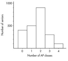
Sometimes, instead of labeling the vertical axis with frequencies, it is more convenient or more meaningful to use relative frequencies, that is, frequencies divided by the total number in the population. In this example, divide the “number of seniors” by the total number in the population.
Number of AP classes | Frequency | Relative frequency |
|---|---|---|
0 | 400 | 400/2200 = 0.18 |
1 | 500 | 500/2200 = 0.23 |
2 | 900 | 900/2200 = 0.41 |
3 | 300 | 300/2200 = 0.14 |
4 | 100 | 100/2200 = 0.05 |
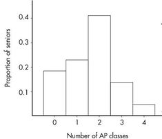
Note that the shape of the histogram is the same whether the vertical axis is labeled with frequencies or with relative frequencies. Sometimes we show both frequencies and relative frequencies on the same graph.
Describing the Distribution of a Quantitative Variable
Looking at a graphical display, we see that two important aspects of the overall pattern are:
Center - which separates the values (or area under the curve in the case of a histogram) roughly in half.
Spread - that is, the scope of the values from smallest to largest.
Other important aspects of the overall pattern are:
clusters - which show natural subgroups into which the values fall. (Example - the salaries of teachers in Ithaca, NY, fall into three overlapping clusters: one for public school teachers, a higher one for Ithaca College professors, and an even higher one for Cornell University professors.)
gaps - which show holes where no values fall. (Example - the Office of the Dean sends letters to students being put on the honor roll and to those being put on academic warning for low grades; thus, the GPA distribution of students receiving letters from the Dean has a huge middle gap.)
➥ Example 1.3
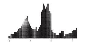
Hodgkin’s lymphoma is a cancer of the lymphatic system, the system that drains excess fluid from the blood and protects against infection. Consider the following histogram:
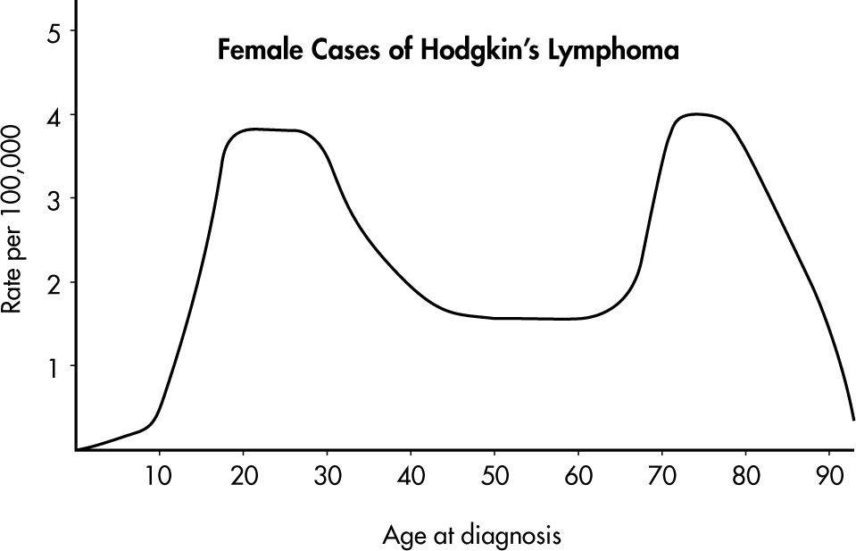
Simply saying that the average age at diagnosis for female cases is around 50 clearly misses something. The distribution of ages at diagnosis for female cases of Hodgkin’s lymphoma is bimodal with two distinct clusters, centered at 25 and 75.
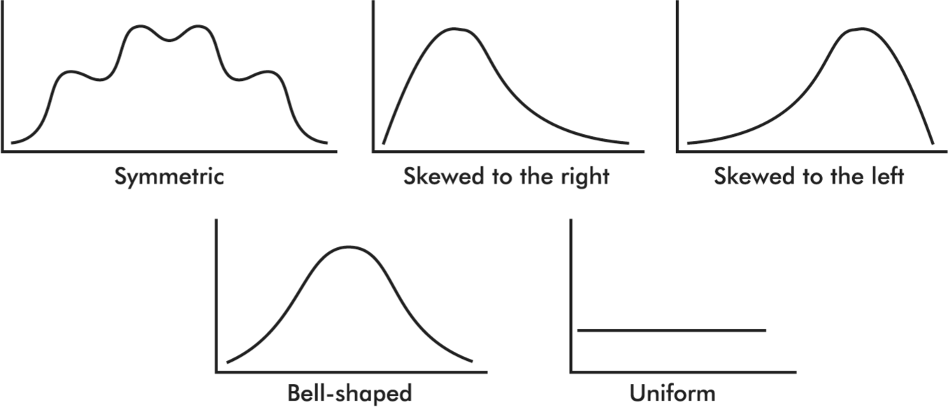
Distributions come in an endless variety of shapes; however, certain common patterns are worth special mention:
A distribution with one peak is called unimodal and a distribution with two peaks is called bimodal.
A symmetric distribution is one in which the two halves are mirror images of each other.
A distribution is skewed to the right if it spreads far and thinly toward the higher values.
A distribution is skewed to the left if it spreads far and thinly toward the lower values.
A bell-shaped distribution is symmetric with a center mound and two sloping tails.
A distribution is uniform if its histogram is a horizontal line.
Summary Statistics for a Quantitative Variable
Descriptive Statistics - The presentation of data, including summarizations and descriptions, and involving such concepts as representative or average values, measures of variability, positions of various values, and the shape of a distribution.
Inferential statistics - the process of drawing inferences from limited data, a subject discussed in later units.
Average has come to mean a representative score or a typical value or the center of a distribution.
Two primary ways of denoting the "center" of a distribution:
The median - which is the middle number of a set of numbers arranged in numerical order.
The mean - which is found by summing items in a set and dividing by the number of items.
➥ Example 1.4
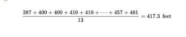
Consider the following set of home run distances (in feet) to center field in 13 ballparks: {387, 400, 400, 410, 410, 410, 414, 415, 420, 420, 421, 457, 461}. What is the average?
Solution: The median is 414 (there are six values below 414 and six values above), while the mean is
The arithmetic mean - is most important for statistical inference and analysis.
The mean of a whole population (the complete set of items of interest) is often denoted by the Greek letter µ (mu).
The mean of a sample (a part of a population) is often denoted by x̄.
➥ Example 1.5
Suppose the salaries of six employees are $3,000, $7,000, $15,000, $22,000, $23,000, and $38,000, respectively.
a. What is the mean salary?
b. What will the new mean salary be if everyone receives a $3000 increase?
c. What if instead everyone receives a 10% raise?
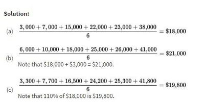
Example 1.5 illustrates how adding the same constant to each value increases the mean by the same amount. Similarly, multiplying each value by the same constant multiplies the mean by the same amount.
Variability - is the single most fundamental concept in statistics and is the key to understanding statistics.
Four primary ways of describing variability, or dispersion:
Range - the difference between the largest and smallest values, or maximum minus minimum.
Interquartile Range (IQR) - the difference between the largest and smallest values after removing the lower and upper quartiles (i.e., IQR is the range of the middle 50%); that is IQR = Q3 – Q1 = 75th percentile minus 25th percentile.
Variance - the average of the squared differences from the mean.
Standard Deviation - the square root of the variance. The standard deviation gives a typical distance that each value is away from the mean.
➥ Example 1.6
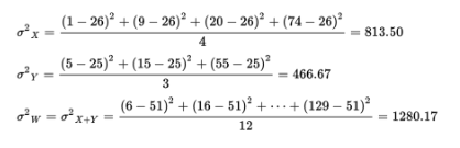
The ages of the 12 mathematics teachers at a high school are {24, 25, 25, 29, 34, 37, 41, 42, 48, 48, 54, 61}.
The mean is
What are the measures of variability?
Solution:
Range: Maximum minus minimum = 61 – 24 = 37 years
Interquartile range: Method 1: Remove the data that makes up the lower quarter {24, 25, 25} and the data that makes up the upper quarter {48, 54, 61}. This leaves the data from the middle two quarters {29, 34, 37, 41, 42, 48}. Subtract the minimum from the maximum of this set: 48 – 29 = 19 years.
Method 2: The median of the lower half of the data is
![]()
and the median of the upper half of the data is
![]()
Subtract Q1 from Q3: 48 – 27 = 21 years.
Variance:
Standard Deviation:
The mathematics teachers’ ages typically vary by about 11.655 years from the mean of 39 years.
Three important, recognized procedures for designating position:
Simple ranking - which involves arranging the elements in some order and noting where in that order a particular value falls.
Percentile ranking - which indicates what percentage of all values fall at or below the value under consideration.
The z-score - which states very specifically the number of standard deviations a particular value is above or below the mean.
Graphical Representations of Summary Statistics
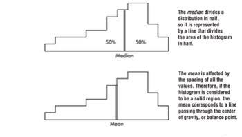
The above distribution, spread thinly far to the low side, is said to be skewed to the left. Note that in this case the mean is usually less than the median. Similarly, a distribution spread thinly far to the high side is skewed to the right, and its mean is usually greater than its median.
➥ Example 1.7
Suppose that the faculty salaries at a college have a median of $82,500 and a mean of $88,700. What does this indicate about the shape of the distribution of the salaries?
Solution: The median is less than the mean, and so the salaries are probably skewed to the right. There are a few highly paid professors, with the bulk of the faculty at the lower end of the pay scale.
➥ Example 1.8
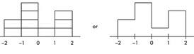
Suppose we are asked to construct a histogram from these data:
z-score: | –2 | –1 | 0 | 1 | 2 |
|---|---|---|---|---|---|
Percentile ranking: | 0 | 20 | 60 | 70 | 100 |
We note that the entire area is less than z-score +2 and greater than z-score −2. Also, 20% of the area is between z-scores −2 and −1, 40% is between −1 and 0, 10% is between 0 and 1, and 30% is between 1 and 2. Thus the histogram is as follows:
Now suppose we are given four in-between z-scores as well:
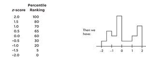
With 1,000 z-scores perhaps the histogram would look like:
The height at any point is meaningless; what is important is relative areas.
In the final diagram above, what percentage of the area is between z-scores of +1 and +2?
What percent is to the left of 0?
Solution:
Still 30%.
Still 60%.
Comparing Distributions of a Quantitative Variable
Four examples showing comparisons involving back-to-back stemplots, side-by-side histograms, parallel boxplots, and cumulative frequency plots :
➥ Example 1.9
The numbers of wins for the 30 NBA teams at the end of the 2018–2019 season is shown in the following back-to-back stemplot.
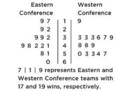
When comparing shape, center, spread, and unusual features, we have:
Shape: The distribution of wins in the Eastern Conference (EC) is roughly bell-shaped, while the distribution of wins in the Western Conference (WC) is roughly uniform with a low outlier.
Center: Counting values (8th out of 15) gives medians of mEC = 41 and mWC = 49. Thus, the WC distribution of wins has the greater center.
Spread: The range of the EC distribution of wins is 60 − 17 = 43, while the range of the WC distribution of wins is 57 − 19 = 38. Thus, the EC distribution of wins has the greater spread. Unusual features: The WC distribution has an apparent outlier at 19 and a gap between 19 and 33, which is different than the EC distribution that has no apparent outliers or gaps.
➥ Example 1.10
Two surveys, one of high school students and one of college students, asked students how many hours they sleep per night. The following histograms summarize the distributions.
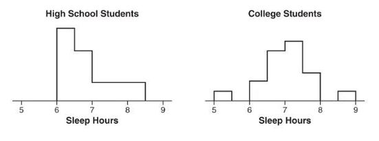
When comparing shape, center, spread, and unusual features, we have the following:
Shape: The distribution of sleep hours in the high school student distribution is skewed right, while the distribution of sleep hours in the college student distribution is unimodal and roughly symmetric.
Center: The median sleep hours for the high school students (between 6.5 and 7) is less than the median sleep hours for the college students (between 7 and 7.5).
Spread: The range of the college student sleep hour distribution is greater than the range of the high school student sleep hour distribution.
Unusual features: The college student sleep hour distribution has two distinct gaps, 5.5 to 6 and 8 to 8.5, and possible low and high outliers, while the high school student sleep hour distribution doesn’t clearly show possible gaps or outliers.
➥ Example 1.11
The following are parallel boxplots showing the daily price fluctuations of a particular common stock over the course of 5 years. What trends do the boxplots show?
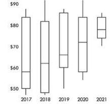
Solution: The parallel boxplots show that from year to year the median daily stock price has steadily risen 20 points from about $58 to about $78, the third quartile value has been roughly stable at about $84, the yearly low has never decreased from that of the previous year, and the interquartile range has never increased from one year to the next. Note that the lowest median stock price was in 2017, and the highest was in 2021. The smallest spread (as measured by the range) in stock prices was in 2021, and the largest was in 2018. None of the price distributions shows an outlier.
➥ Example 1.12
The graph below compares cumulative frequency plotted against age for the U.S. population in 1860 and in 1980.
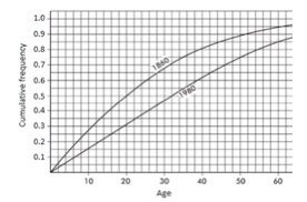
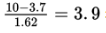
How do the medians and interquartile ranges compare?
Solution: Looking across from 0.5 on the vertical axis, we see that in 1860 half the population was under the age of 20, while in 1980 all the way up to age 32 must be included to encompass half the population. Looking across from 0.25 and 0.75 on the vertical axis, we see that for 1860, Q1 = 9 and Q3 = 35 and so the interquartile range is 35 − 9 = 26 years, while for 1980, Q1 = 16 and Q3 = 50 and so the interquartile range is 50 − 16 = 34 years. Thus, both the median and the interquartile range were greater in 1980 than in 1860.
The Normal Distribution
Normal distribution is valuable for providing a useful model in describing various natural phenomena. It can be used to describe the results of many sampling procedures.
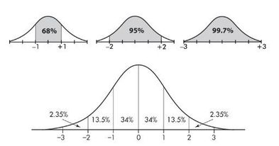
The normal distribution curve is bell-shaped and symmetric and has an infinite base.
The mean of a normal distribution is equal to the median and is located at the center. There is a point on each side where the slope is steepest. These two points are called points of inflection, and the distance from the mean to either point is precisely equal to one standard deviation. Thus, it is convenient to measure distances under the normal curve in terms of z-scores.
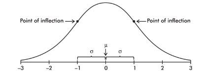
The empirical rule (also called the 68-95-99.7 rule) applies specifically to normal distributions. In this case, about 68% of the values lie within 1 standard deviation of the mean, about 95% of the values lie within 2 standard deviations of the mean, and about 99.7% of the values lie within 3 standard deviations of the mean.
➥ Example 1.13
Suppose that taxicabs in New York City are driven an average of 75,000 miles per year with a standard deviation of 12,000 miles. What information does the empirical rule give us?
Solution: Assuming that the distribution is roughly normal, we can conclude that approximately 68% of the taxis are driven between 63,000 and 87,000 miles per year, approximately 95% are driven between 51,000 and 99,000 miles, and virtually all are driven between 39,000 and 111,000 miles.
Unit 2: Exploring Two-Variable Data
Two Categorical Variables
Qualitative data often encompass two categorical variables that may or may not have a dependent relationship. These data can be displayed in a two-way table (also called a contingency table).
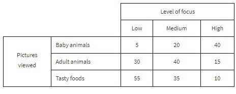
➥ Example 2.1
The Cuteness Factor: A Japanese study had 250 volunteers look at pictures of cute baby animals, adult animals, or tasty-looking foods, before testing their level of focus in solving puzzles.
The grand total of all cell values, 250 in this example, is called the table total.
Pictures viewed is the row variable, whereas level of focus is the column variable.
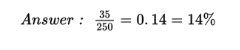
What percent of the people in the survey viewed tasty foods and had a medium level of focus?
The standard method of analyzing the table data involves first calculating the totals for each row and each column.
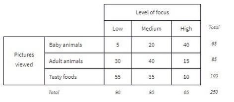
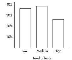
These totals are placed in the right and bottom margins of the table and thus are called marginal frequencies (or marginal totals). These marginal frequencies can then be put in the form of proportions or percentages. The marginal distribution of the level of focus is:
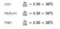
This distribution can be displayed in a bar graph as follows:
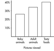
Similarly, we can determine the marginal distribution for the pictures viewed:
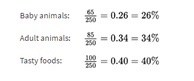
The representative bar graph is:
Two Quantitative Variables
Many important applications of statistics involve examining whether two or more quantitative (numerical) variables are related to one another.
These are also called bivariate quantitative data sets.
Scatterplot - gives an immediate visual impression of a possible relationship between two variables, while a numerical measurement, called the correlation coefficient - often used as a quantitative value of the strength of a linear relationship. In either case, evidence of a relationship is not evidence of causation.
➥ Example 2.2
Comic books heroes and villains can be compared with regard to various attributes. The scatterplot below looks at speed (measured on a 20-point scale) versus strength (measured on a 50-point scale) for 17 such characters. Does there appear to be a linear association?
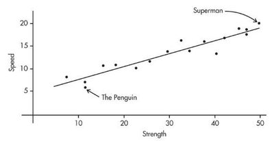
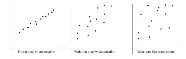
Positively associated- When larger values of one variable are associated with larger values of a second variable.
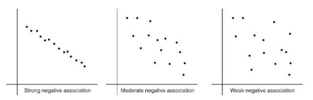
Negatively associated - When larger values of one are associated with smaller values of the other, the variables are called negatively associated.
The strength of the association is gauged by how close the plotted points are to a straight line.
To describe a scatterplot you must consider form (linear or nonlinear), direction (positive or negative), strength (weak, moderate, or strong), and unusual features (such as outliers and clusters). As usual, all answers must also mention context.
Correlation
Correlation measures the strength of only a linear relationship.
Correlation, designated by r, has the formula in terms of the means and standard deviations of the two variables.
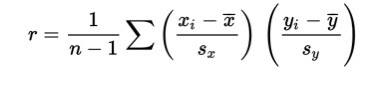
The correlation formula gives the following:
The formula is based on standardized scores (z**-scores**), and so changing units does not change the correlation r.
Since the formula does not distinguish between which variable is called x and which is called y, interchanging the variables (on the scatterplot) does not change the value of the correlation r.
The division in the formula gives that the correlation r is unit-free.
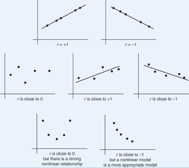
The value of r always falls between −1 and +1, with −1 indicating perfect negative correlation and +1 indicating perfect positive correlation. It should be stressed that a correlation at or near zero does not mean there is not a relationship between the variables; there may still be a strong nonlinear relationship. Additionally, a correlation close to −1 or +1 does not necessarily mean that a linear model is the most appropriate model.
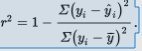
r2 (called the coefficient of determination) - is the ratio of the variance of the predicted values ŷ to the variance of the observed values y.
That is, there is a partition of the y-variance, and r2 is the proportion of this variance that is predictable from a knowledge of x.
We can say that r2 gives the percentage of variation in the response variable, y, that is explained by the variation in the explanatory variable, x. Or we can say that r2 gives the percentage of variation in y that is explained by the linear regression model between x and y. In any case, always interpret r2 in context of the problem. Remember when calculating r from r2 that r may be positive or negative, and that r will always take the same sign as the slope.
Alternatively, r2 is 1 minus the proportion of unexplained variance:
➥ Example 2.3
The correlation between Total Points Scored and Total Yards Gained for the 2021 season among a set of college football teams is r = 0.84. What information is given by the coefficient of determination?
Solution: r2 = (0.84)2 = 0.7056. Thus, 70.56% of the variation in Total Points Scored can be accounted for by (or predicted by or explained by) the linear relationship between Total Points Scored and Total Yards Gained. The other 29.44% of the variation in Total Points Scored remains unexplained.
Least Squares Regression
What is the best-fitting straight line that can be drawn through a set of points?
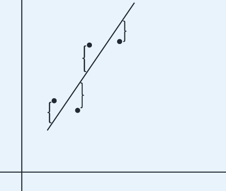
By best-fitting straight line we mean the straight line that minimizes the sum of the squares of the vertical differences between the observed values and the values predicted by the line.
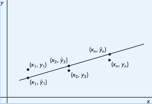
That is, in the above figure, we wish to minimize
![]()
It is reasonable, intuitive, and correct that the best-fitting line will pass through ( x̄,ȳ), where x̄ and ȳare the means of the variables X and Y. Then, from the basic expression for a line with a given slope through a given point, we have:
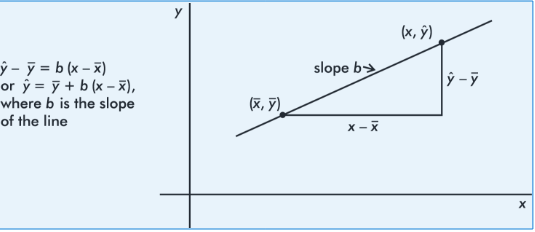
The slope b can be determined from the formula
![]()
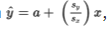
where r is the correlation and sx and sy are the standard deviations of the two sets. That is, each standard deviation change in x results in a change of r standard deviations in ŷ. If you graph z-scores for the y-variable against z-scores for the x-variable, the slope of the regression line is precisely r, and in fact, the linear equation becomes,
![]()
Example 2.4
A sociologist conducts a survey of 15 teens. The number of "close friends" and the number of times Facebook is checked every evening are noted for each student. Letting X and Y represent the number of close friends and the number of Facebook checks, respectively, gives:
X: | 25 | 23 | 30 | 25 | 20 | 33 | 18 | 21 | 22 | 30 | 26 | 26 | 27 | 29 | 20 |
|---|---|---|---|---|---|---|---|---|---|---|---|---|---|---|---|
Y: | 10 | 11 | 14 | 12 | 8 | 18 | 9 | 10 | 10 | 15 | 11 | 15 | 12 | 14 | 11 |
Identify the variables.
Draw a scatterplot.
Describe the scatterplot.
What is the equation of the regression line? Interpret the slope in context.
Interpret the coefficient of determination in context.
Predict the number of evening Facebook checks for a student with 24 close friends.
Solution:
The explanatory variable, X, is the number of close friends and the response variable, Y, is the number of evening Facebook checks.
Plotting the 15 points (25, 10), (23, 11), . . . , (20, 11) gives an intuitive visual impression of the relationship:
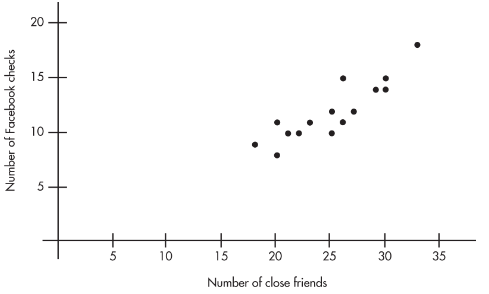
The relationship between the number of close friends and the number of evening Facebook checks appears to be linear, positive, and strong.
Calculator software gives ŷ= -1.73 + 0.5492x , where x is the number of close friends and y is the number of evening Facebook checks. We can instead write the following:

The slope is 0.5492. Each additional close friend leads to an average of 0.5492 more evening Facebook checks.
Calculator software gives r = 0.8836, so r2 = 0.78. Thus, 78% of the variation in the number of evening Facebook checks is accounted for by the variation in the number of close friends.
–1.73 + 0.5492(24) = 11.45 evening Facebook checks. Students with 24 close friends will average 11.45 evening Facebook checks.
Residuals
Residual - difference between an observed and a predicted value.
When the regression line is graphed on the scatterplot, the residual of a point is the vertical distance the point is from the regression line.
A positive residual means the linear model underestimated the actual response value.
Negative residual means the linear model overestimated the actual response value.
➥ Example 2.4
We calculate the predicted values from the regression line in Example 2.13 and subtract from the observed values to obtain the residuals:
x | 30 | 90 | 90 | 75 | 60 | 50 |
|---|---|---|---|---|---|---|
y | 185 | 630 | 585 | 500 | 430 | 400 |
ŷ | 220.3 | 613.3 | 613.3 | 515.0 | 416.8 | 351.3 |
y-ŷ | –35.3 | 16.7 | –28.3 | –15.0 | 13.2 | 48.7 |
Note that the sum of the residuals is
–35.3 + 16.7 – 28.3 – 15.0 + 13.2 + 48.7 = 0
The above equation is true in general; that is, the sum and thus the mean of the residuals is always zero.
Outliers, Influential Points, and Leverage
In a scatterplot, regression outliers are indicated by points falling far away from the overall pattern. That is, outliers are points with relatively large discrepancies between the value of the response variable and a predicted value for the response variable.
In terms of residuals, a point is an outlier if its residual is an outlier in the set of residuals.
➥ Example 2.5
A scatterplot of grade point average (GPA) versus weekly television time for a group of high school seniors is as follows:
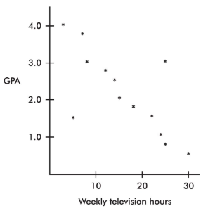
By direct observation of the scatterplot, we note that there are two outliers: one person who watches 5 hours of television weekly yet has only a 1.5 GPA, and another person who watches 25 hours weekly yet has a 3.0 GPA. Note also that while the value of 30 weekly hours of television may be considered an outlier for the television hours variable and the 0.5 GPA may be considered an outlier for the GPA variable, the point (30, 0.5) is not an outlier in the regression context because it does not fall off the straight-line pattern.
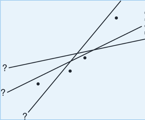
Influential Scores - Scores whose removal would sharply change the regression line. Sometimes this description is restricted to points with extreme x-values. An influential score may have a small residual but still have a greater effect on the regression line than scores with possibly larger residuals but average x-values.
➥ Example 2.
Consider the following scatterplot of six points and the regression line:
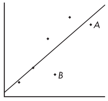
The heavy line in the scatterplot on the left below shows what happens when point A is removed, and the heavy line in the scatterplot on the right below shows what happens when point B is removed.
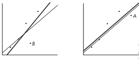
Note that the regression line is greatly affected by the removal of point A but not by the removal of point B. Thus, point A is an influential score, while point B is not. This is true in spite of the fact that point A is closer to the original regression line than point B.
A point is said to have high leverage if its x-value is far from the mean of the x-values. Such a point has the strong potential to change the regression line. If it happens to line up with the pattern of the other points, its inclusion might not influence the equation of the regression line, but it could well strengthen the correlation and r2, the coefficient of determination.
➥ Example 2.7
Consider the four scatterplots below, each with a cluster of points and one additional point separated from the cluster.
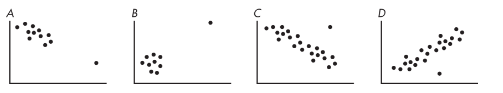
In A, the additional point has high leverage (its x-value is much greater than the mean x-value), has a small residual (it fits the overall pattern), and does not appear to be influential (its removal would have little effect on the regression equation).
In B, the additional point has high leverage (its x-value is much greater than the mean x-value), probably has a small residual (the regression line would pass close to it), and is very influential (removing it would dramatically change the slope of the regression line to close to 0).
In C, the additional point has some leverage (its x-value is greater than the mean x-value but not very much greater), has a large residual compared to other residuals (so it's a regression outlier), and is somewhat influential (its removal would change the slope to more negative).
In D, the additional point has no leverage (its x-value appears to be close to the mean x-value), has a large residual compared to other residuals (so it's a regression outlier), and is not influential (its removal would increase the y-intercept very slightly and would have very little if any effect on the slope).
More on Regression
The regression equation
![]() has important implications.
has important implications.
If the correlation r = +1, then
, and for each standard deviation sx increase in x, the predicted y-value increases by Sy.
If, for example, r = +0.4, then
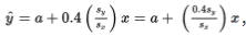
, and for each standard deviation sx increase in x, the predicted y-value increases by 0.4 Sy.
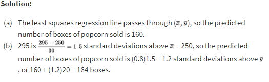
➥ Example 2.8
Suppose x = attendance at a movie theater, y = number of boxes of popcorn sold, and we are given that there is a roughly linear relationship between x and y. Suppose further we are given the summary statistics:

When attendance is 250, what is the predicted number of boxes of popcorn sold?
When attendance is 295, what is the predicted number of boxes of popcorn sold?
The regression equation for predicting x from y has the slope:
![]()
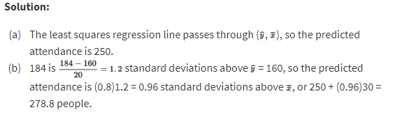
➥ Example 2.9
Use the same attendance and popcorn summary statistics from Example 2.24 above.
When 160 boxes of popcorn are sold, what is the predicted attendance?
When 184 boxes of popcorn are sold, what is the predicted attendance?
Transformations to Achieve Linearity
The nonlinear model can sometimes be revealed by transforming one or both of the variables and then noting a linear relationship. Useful transformations often result from using the log or ln buttons on your calculator to create new variables.
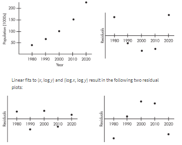
➥ Example 2.10
Consider the following years and corresponding populations:
Year, x: | 1980 | 1990 | 2000 | 2010 | 2020 |
|---|---|---|---|---|---|
Population (1000s), y: | 44 | 65 | 101 | 150 | 230 |
![]()
So, 94.3% of the variability in population is accounted for by the linear model. However, the scatterplot and residual plot indicate that a nonlinear relationship would be an even stronger model.
Unit 3: Collecting Data
Retrospective Versus Prospective Observational Studies
Observational studies aim to gather information about a population without disturbing the population.
Retrospective studies look backward, examining existing data.
Prospective studies watch for outcomes, tracking individuals into the future.
➥ Example 3.1
Retrospective studies of the 2014–2016 Ebola epidemic in West Africa have looked at the timing, numbers, and locations of reported cases and have tried to understand how the outbreak spread. There is now much better understanding of transmission through contact with bodily fluids of infected people. Several prospective studies involve ongoing surveillance to see how experience and tools to rapidly identify cases will now limit future epidemics.
Advantages and Disadvantages
Retrospective studies tend to be smaller scale, quicker to complete, and less expensive. In cases such as addressing diseases with low incidence, the study begins right from the start with people who have already been identified. However, researchers have much less control, usually having to rely on past record keeping of others. Furthermore, the existing data will often have been gathered for other purposes than the topic of interest. Then there is the problem of subjects' inaccurate memories and possible biases.
Prospective studies usually have greater accuracy in data collection and are less susceptible to recall error from subjects. Researchers do their own record keeping and can monitor exactly what variables they are interested in. However, these studies can be very expensive and time consuming, as they often follow large numbers of subjects for a long time.
Bias
The one thing that most quickly invalidates a sample and makes obtaining useful information and drawing meaningful conclusions impossible.
Sampling method - is biased if in some critical way it consistently results in samples that do not represent the population**.** This typically leads to certain responses being repeatedly favored over others.
Sampling bias - is a property of the sampling method, not of any one sample generated by the method.
Voluntary response surveys - are based on individuals who choose to participate, typically give too much emphasis to people with strong opinions, and undersample people who don’t care much about a topic.
Although a voluntary response survey may be easy and inexpensive to conduct, the sample is likely to be composed of strongly opinionated people, especially those with negative opinions on a subject.
Convenience surveys - are based on choosing individuals who are easy to reach. These surveys tend to produce data highly unrepresentative of the entire population.
Although convenience samples may allow a researcher to conduct a survey quickly and inexpensively, generalizing from the sample to a population is almost impossible.
Undercoverage bias - happens when there is inadequate representation, and thus some groups in the population are left out of the process of choosing the sample.
Response bias - occurs when the question itself can lead to misleading results because people don’t want to be perceived as having unpopular or unsavory views or don’t want to admit to having committed crimes.
Nonresponse bias - where there are low response rates, occurs when individuals chosen for the sample can’t be contacted or refuse to participate, and it is often unclear which part of the population is responding.
Quota sampling bias - where interviewers are given free choice in picking people in the (problematic, if not impossible) attempt to pick representatively with no randomization, is a recipe for disaster.
Question wording bias - can occur when nonneutral or poorly worded questions lead to very unrepresentative responses or even when the order in which questions are asked makes a difference.
➥Example 3.2
The Military Times, in collaboration with the Institute for Veterans and Military Families at Syracuse University, conducted a voluntary and confidential online survey of U.S. service members who were readers of the Military Times. Their military status was verified through official Defense Department email addresses. What were possible sources of bias?
Solution: First, voluntary online surveys are very suspect because they typically overcount strongly opinionated people. Second, undercoverage bias is likely because only readers of the Military Times took part in the survey. Note that response bias was probably not a problem because the survey was confidential.
Sampling Methods
Census - Collecting data from every individual in a population.
How can we increase our chance of choosing a representative sample?
One technique is to write the name of each member of the population on a card, mix the cards thoroughly in a large box, and pull out a specified number of cards. This method gives everyone in the population an equal chance of being selected as part of the sample. Unfortunately, this method is usually too time-consuming, and bias might still creep in if the mixing is not thorough.
A simple random sample (SRS), one in which every possible sample of the desired size has an equal chance of being selected, can be more easily obtained by assigning a number to everyone in the population and using a random digit table or having a computer generate random numbers to indicate choices.
➥ Example 3.3
Suppose 80 students are taking an AP Statistics course and the teacher wants to pick a sample of 10 students randomly to try out a practice exam. She can make use of a random number generator on a computer. Assign the students numbers 1, 2, 3, …, 80. Use a computer to generate 10 random integers between 1 and 80 without replacement, that is, throw out repeats. The sample consists of the students with assigned numbers corresponding to the 10 unique computer-generated numbers.
An alternative solution:
is to first assign the students numbers 01, 02, 03, . . ., 80. While reading off two digits at a time from a random digit table, she ignores any numbers over 80, ignores 00, and ignores repeats, stopping when she has a set of 10. If the table began 75425 56573 90420 48642 27537 61036 15074 84675, she would choose the students numbered 75, 42, 55, 65, 73, 04, 27, 53, 76, and 10. Note that 90 and 86 are ignored because they are over 80. Note that the second and third occurrences of 42 are ignored because they are repeats.
Advantages of simple random sampling include the following:
The simplicity of simple random sampling makes it relatively easy to interpret data collected.
This method requires minimal advance knowledge of the population other than knowing the complete sampling frame.
Simple random sampling allows us to make generalizations (i.e., statistical inferences) from the sample to the population.
Among the major parameters with which we will work, simple random sampling tends to be unbiased, that is, when repeated many times, it gives sample statistics that are centered around the true parameter value.
Disadvantages of simple random sampling include the following:
The need for a list of all potential subjects can be a formidable task.
Although simple random sampling is a straightforward procedure to understand, it can be difficult to execute, especially if the population is large. For example, how would you obtain a simple random sample of students from the population of all high school students in the United States?
The need to repeatedly contact nonrespondents can be very time-consuming.
Important groups may be left out of the sample when using this method.
Other sampling methods available:
Stratified sampling - involves dividing the population into homogeneous groups called strata, then picking random samples from each of the strata, and finally combining these individual samples into what is called a stratified random sample. (For example, we can stratify by age, gender, income level, or race; pick a sample of people from each stratum; and combine to form the final sample.)
Advantages of stratified sampling include the following:
Samples taken within a stratum have reduced variability, which means the resulting estimates are more precise than when using other sampling methods.
Important differences among groups can become more apparent.
Disadvantages of stratified sampling include the following:
Like an SRS, this method might be difficult to implement with large populations.
Forcing subdivisions when none really exist is meaningless.
Cluster sampling - involves dividing the population into heterogeneous groups called clusters and then picking everyone or everything in a random selection of one or more of the clusters. (For example, to survey high school seniors, we could randomly pick several senior class homerooms in which to conduct our study and sample all students in those selected homerooms.)
Advantages of cluster sampling include the following:
Clusters are often chosen for ease, convenience, and quickness.
With limited fixed funds, cluster sampling usually allows for a larger sample size than do other sampling methods.
Disadvantages of cluster sampling include the following:
With a given sample size, cluster sampling usually provides less precision than either an SRS or a stratified sample provides.
If the population doesn’t have natural clusters and the designated clusters are not representative of the population, selection could easily result in a biased sample.
Systematic sampling - is a relatively simple and quick method. It involves listing the population in some order (for example, alphabetically), choosing a random point to start, and then picking every tenth (or hundredth, or thousandth, or kth) person from the list. This gives a reasonable sample as long as the original order of the list is not in any way related to the variables under consideration.
An advantage of systematic sampling is that if similar members in the list are grouped together, we can end up with a kind of stratified sample, only more easily implemented.
A disadvantage of systematic sampling is that if the list happens to have a periodic structure similar to the period of the sampling, a very biased sample could result.
➥ Example 3.4
Suppose a sample of 100 high school students from a Chicago school of size 5000 is to be chosen to determine their views on whether they think the Cubs will win another World Series this century. One method would be to have each student write his or her name on a card, put the cards into a box, have the principal reach in and pull out 100 cards, and then choose the names on those cards to be the sample. However, questions could arise regarding how well the cards are mixed. For example, how might the outcome be affected if all students in one PE class toss their names in at the same time so that their cards are clumped together? A second method would be to number the students 1 through 5000, and use a random number generator to pick 100 unique (throw out repeats) numbers between 1 and 5000. The sample is then the students whose numbers correspond to the 100 generated numbers. A third method would be to assign each student a number from 0001 to 5000 and use a random digit table, picking out four digits at a time, ignoring repeats, 0000, and numbers over 5000, until a unique set of 100 numbers are picked. Then choose the students corresponding to the selected 100 numbers. What are alternative procedures?
Solution: From a list of the students, the surveyor could choose a random starting name and then simply note every 50th name (systematic sampling). Since students in each class have certain characteristics in common, the surveyor could use a random selection method to pick 25 students from each of the separate lists of freshmen, sophomores, juniors, and seniors (stratified sampling). If each homeroom has a random mix of 20 students from across all grade levels, the surveyor could randomly pick five homerooms with the sample consisting of all the students in these five rooms (cluster sampling).
Sampling Variability
Sampling variability - also called sampling error, is naturally present. This variability can be described using probability; that is, we can say how likely we are to have a certain size error. Generally, the associated probabilities are smaller when the sample size is larger.
➥ Example 3.5
Suppose we are trying to estimate the mean age of high school teachers and have four methods of choosing samples. We choose 10 samples using each method. Later we find the true mean, μ = 42. Plots of the results of each sampling method are given below.
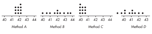
Method A exhibits high accuracy and high precision.
Method B exhibits high accuracy and low precision.
Method C exhibits low accuracy and high precision.
Method D exhibits low accuracy and low precision. Low accuracy (not centered at the right place) indicates probable bias in the selection method.
Note that shape and variability in distributions are completely irrelevant to the issue of sampling bias. Sampling bias is focused on the center of the distribution.
Experiments Versus Observational Studies
Observational Studies | Experiments |
|---|---|
Observe and measure without influencing | Impose treatments and measure responses |
Can only show associations | Can suggest cause-and-effect relationships |
Use of random sampling in order to be able to generalize to a population | Use of random assignment to minimize the effect of confounding variables |
Usually less expensive and less time-consuming | Can be expensive and time-consuming |
Use of strata, and randomization within strata, for greater accuracy and to reduce variability | Use of blocks, and randomization within blocks, to control for certain variables |
Possible ethical concerns over imposing certain treatments | |
Use of blinding and double-blinding |
➥ Example 3.6
A study is to be designed to determine whether a particular commercial review course actually helps raise SAT scores among students attending a particular high school. How could an observational study be performed? An experiment? Which is more appropriate here?
Solution:
An observational study would interview students at the school who have taken the SAT exam, asking whether or not they took the review course, and then the SAT results of those who have and have not taken the review course would be compared.
An experiment performed on students at the school who are planning to take the SAT exam would use chance to randomly assign some students to take the review course while others to not take the course and would then compare the SAT results of those who have and have not taken the review course.
The experimental approach is more appropriate here. With the observational study, there could be many explanations for any SAT score difference noted between those who took the course and those who didn’t. For example, students who took the course might be the more serious high school students. Higher score results might be due to their more serious outlook and have nothing to do with taking the course. The experiment tries to control for confounding variables by using random assignment to make the groups taking and not taking the course as similar as possible except for whether or not the individuals take the course.
The Language of Experiments
Experimental units - An experiment is performed on objects.
Subjects - If the units are people.
Experiments involve explanatory variables, called factors, that are believed to have an effect on response variables. A group is intentionally treated with some level of the explanatory variable, and the outcome of the response variable is measured.
➥ Example 3.7
In an experiment to test exercise and blood pressure reduction, volunteers are randomly assigned to participate in either 0, 1, or 2 hours of exercise per day for 5 days over the next 6 months. What is the explanatory variable with the corresponding levels, and what is the response variable?
Solution: The explanatory variable, hours of exercise, is being implemented at three levels: 0, 1, and 2 hours a day. The response variable is not specified but could be the measured change in either systolic or diastolic blood pressure readings after 6 months.
Suppose the volunteers were further randomly assigned to follow either the DASH (Dietary Approaches to Stop Hypertension) or the TLC (Therapeutic Lifestyle Changes) diet for the 6 months. There would then be two factors, hours of exercise with three levels and diet plan with two levels, and a total of six treatments (DASH diet with 0 hours daily exercise, DASH with 1 hour exercise, DASH with 2 hours exercise, TLC diet with 0 hours daily exercise, TLC with 1 hour exercise, and TLC with 2 hours exercise).
In an experiment, there is often a control group to determine if the treatment of interest has an effect. There are several types of control groups.
A control group can be a collection of experimental units not given any treatment, or g__iven the current treatment__, or given a treatment with an inactive substance (a placebo). When a control group receives the current treatment or a placebo, these count as treatments if asked to enumerate the treatments.
➥ Example 3.8
Sixty patients, ages 5 to 12, all with common warts are enrolled in a study to determine if application of duct tape is as effective as cryotherapy in the treatment of warts. Subjects will receive either cryotherapy (liquid nitrogen applied to each wart for 10 seconds every 2 weeks) for 6 treatments or duct tape occlusion (applied directly to the wart) for 2 months. Describe a completely randomized design.
Solution: Assign each patient a number from 1 to 60. Use a random integer generator on a calculator to pick integers between 1 and 60, throwing away repeats, until 30 unique integers have been selected. (Or numbering the patients with two-digit numbers from 01 to 60, use a random number table, reading off two digits at a time, ignoring repeats, 00, and numbers over 60, until 30 unique numbers have been selected.) The 30 patients corresponding to the 30 selected integers will be given the cryotherapy treatment. (A third design would be to put the 60 names on identical slips of paper, put the slips in a hat, mix them well, and then pick out 30 slips, without replacement, with the corresponding names given cryotherapy.) The remaining 30 patients will receive the duct tape treatment. At the end of the treatment schedules, compare the proportion of each group that had complete resolution of the warts being studied.
Placebo Effect - It is a fact that many people respond to any kind of perceived treatment. (For example, when given a sugar pill after surgery but told that it is a strong pain reliever, many people feel immediate relief from their pain.)
Blinding - occurs when the subjects don’t know which of the different treatments (such as placebos) they are receiving.
Double-blinding - is when neither the subjects nor the response evaluators know who is receiving which treatment.
➥ Example 3.9
There is a pressure point on the wrist that some doctors believe can be used to help control the nausea experienced following certain medical procedures. The idea is to place a band containing a small marble firmly on a patient’s wrist so that the marble is located directly over the pressure point. Describe how a double-blind experiment might be run on 50 postoperative patients.
Solution: Assign each patient a number from 1 to 50. Use a random integer generator on a calculator to pick integers between 1 and 50, ignoring repeats, until 25 unique integers have been selected. (Or numbering the patients with two-digit numbers from 01 to 50, from a random number table read off two digits at a time, throwing away repeats, 00, and numbers over 50, until 25 unique numbers have been selected.) Put wristbands with marbles over the pressure point on the patients with these assigned numbers. (A third experimental design would be to put the 50 names on identical slips of paper, put the slips in a hat, mix them well, and then pick out 25 slips, without replacement, with the corresponding names given wristbands with marbles over the pressure point.) Put wristbands with marbles on the remaining patients also, but not over the pressure point. Have a researcher check by telephone with all 50 patients at designated time intervals to determine the degree of nausea being experienced. Neither the patients nor the researcher on the telephone should know which patients have the marbles over the correct pressure point.
A matched pairs design (also called a paired comparison design) - is when two treatments are compared based on the responses of paired subjects, one of whom receives one treatment while the other receives the second treatment. Often the paired subjects are really single subjects who are given both treatments, one at a time in random order.
Replication and Generalizability of Results
One important consideration is the size of the sample: the larger the sample, the more significant the observation. This is the principle of replication. In other words, the treatment should be repeated on a sufficient number of subjects so that real response differences are more apparent.
Replication - refers to having more than one experimental unit in each treatment group, not multiple trials of the same experiment.
Randomization - is critical to minimize the effect of confounding variables. However, in order to generalize experimental results to a larger population (as we try to do in sample surveys), it would also be necessary that the group of subjects used in the experiment be randomly selected from the population.
Inference and Experiments
If the treatments make no difference, just by chance there probably will be some variation.
Something is statistically significant if the probability of it happening just by chance is so small that you’re convinced there must be another explanation.
➥ Example 3.10
Sixty students volunteered to participate in an experiment comparing the effects of coffee, caffeinated cola, and herbal tea on pulse rates. Twenty students are randomly assigned to each of the three treatments. For each student, the change in pulse rate was measured after consuming eight ounces of the treatment beverage. The results are summarized with the parallel boxplots below.
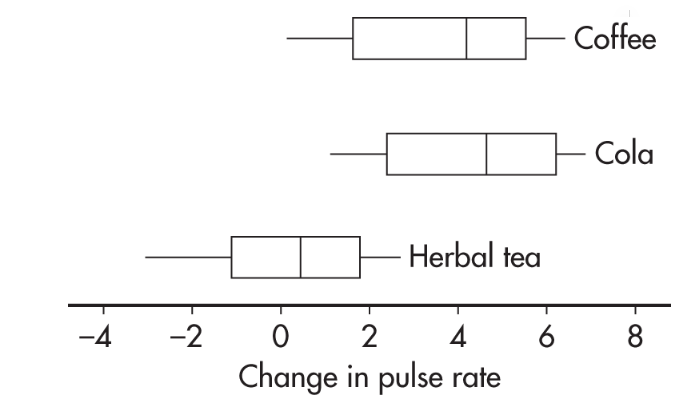
What are reasonable conclusions?
Answer: The median change in pulse rate for the cola drinkers was higher than that for the coffee drinkers; however, looking at the overall spreads, that observed difference does not seem significant. The difference between the coffee and caffeinated cola drinkers with respect to change in pulse rate is likely due to random chance. Now compare the coffee and caffeinated cola drinkers’ results to that of the herbal tea drinkers. While there is some overlap, there is not much. It seems reasonable to conclude the difference is statistically significant; that is, drinking coffee or caffeinated cola results in a greater rise in pulse rate than drinking herbal tea.
Unit 4: Probability, Random Variables, and Probability Distributions
The Law of Large Numbers
Law of large numbers - states that when an experiment is performed a large number of times, the relative frequency of an event tends to become closer to the true probability of the event; that is, probability is long-run relative frequency. There is a sense of predictability about the long run.
The law of large numbers has two conditions:
First, the chance event under consideration does not change from trial to trial.
Second, any conclusion must be based on a large (a very large!) number of observations.
➥ Example 4.1
There are two games involving flipping a fair coin. In the first game, you win a prize if you can throw between 45% and 55% heads. In the second game, you win if you can throw more than 60% heads. For each game, would you rather flip 20 times or 200 times?
Solution: The probability of throwing heads is 0.5. By the law of large numbers, the more times you throw the coin, the more the relative frequency tends to become closer to this probability. With fewer tosses, there is greater chance of wide swings in the relative frequency. Thus, in the first game, you would rather have 200 flips, whereas in the second game, you would rather have only 20 flips.
Basic Probability Rules
➥ Example 4.2
A standard literacy test consists of 100 multiple-choice questions, each with five possible answers. There is no penalty for guessing. A score of 60 is considered passing, and a score of 80 is considered superior. When an answer is completely unknown, test takers employ one of three strategies: guess, choose answer (c), or choose the longest answer. The table below summarizes the results of 1000 test takers.
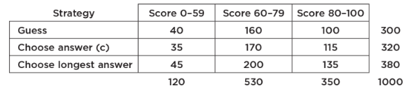
What is the probability that someone in this group uses the “guess” strategy?
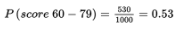
What is the probability that someone in this group scores 60–79?
What is the probability that someone in this group does not score 60–79?
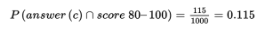
What is the probability that someone in this group chooses strategy “answer (c)” and scores 80–100 (sometimes called the joint probability of the two events)?
What is the probability that someone in this group chooses strategy “longest answer” or scores 0–59?
What is the probability that someone in this group chooses the strategy “guess” given that his or her score was 0–59?
What is the probability that someone in this group scored 80–100 given that the person chose strategy “longest answer”?
Are the strategy “guess” and scoring 0–59 independent events? That is, is whether a test taker used the strategy “guess” unaffected by whether the test taker scored 0–59?
Are the strategy “longest answer” and scoring 80–100 mutually exclusive events? That is, are these two events disjoint and cannot simultaneously occur?
Solution:
![]()
P(does not score 60–79) = 1 − P(score 60–79) = 1 − 0.53 = 0.47

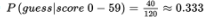

We must check if P (guess|score 0–59) = P(guess). From (f) and (a), we see that these probabilities are not equal (0.333 ≠ 0.3), so the strategy “guess” and scoring 0–59 are not independent events.
longest answer ∩ score 80–100 ≠ Ø and P(longest answer ∩ score 80–100) = 135/1000 ≠ 0, so the strategy “longest answer” and scoring 80–100 are not mutually exclusive events.
Multistage Probability Calculations
➥ Example 4.3
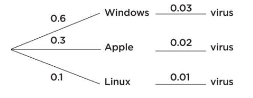
On a university campus, 60%, 30%, and 10% of the computers use Windows, Apple, and Linux operating systems, respectively. A new virus affects 3% of the Windows, 2% of the Apple, and 1% of the Linux operating systems. What is the probability a computer on this campus has the virus?
Solution: In such problems, it is helpful to start with a tree diagram.
We then have:
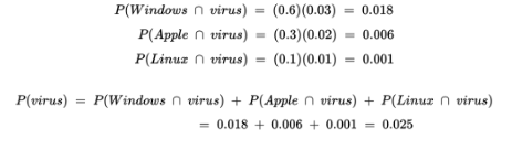
Random Variables, Means (Expected Values), and Standard Deviations
Often each outcome of an experiment has not only an associated probability but also an associated real number.
If X represents the different numbers associated with the potential outcomes of some chance situation, we call X a random variable.
➥ Example 4.4
A charity holds a lottery in which 10,000 tickets are sold at $1 each and with a prize of $7500 for one winner. What is the average result for each ticket holder?
Solution: The actual winning payoff is $7499 because the winner paid $1 for a ticket. Letting X be the payoff random variable, we have:
Outcome | Random Variable X | Probability P(x) |
|---|---|---|
Win | 7499 | 1/10,000 |
Lose | –1 | 9,999/10,000 |
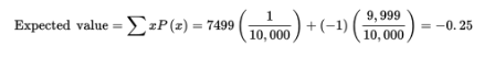
Thus, the average result for each ticket holder is a $0.25 loss. [Alternatively, we can say that the expected payoff to the charity is $0.25 for each ticket sold.]
The mean of this new discrete random variable is ∑(xi − µx)2pi, which is precisely how we define the variance, σ2, of a discrete random variable:
![]()
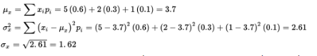
➥ Example 4.5
A highway engineer knows that the workers can lay 5 miles of highway on a clear day, 2 miles on a rainy day, and only 1 mile on a snowy day. Suppose the probabilities are as follows:
Outcome | Random variable X (Miles of highway) | Probability P(x) |
|---|---|---|
Clear | 5 | 0.6 |
Rain | 2 | 0.3 |
Snow | 1 | 0.1 |
What are the mean (expected value), standard deviation, and variance?
Would it be surprising if the workers laid 10 miles of highway one day?
Solution:
In the long run, the workers will lay an average of 3.7 miles of highway per day. The number of miles the workers lay on a randomly selected day will generally vary about 1.62 from the mean of 3.7 miles.
10 is
 standard deviations above the mean, so this would be very surprising!
Means and Variances for Sums and Differences of Sets
When the random variables are independent, there is an easy calculation for finding both the mean and standard deviation of the sum (and difference) of the two random variables.
➥ Example 4.6
A casino offers couples at the hotel free chips by allowing each person to reach into a bag and pull out a card stating the number of free chips. One person’s bag has a set of four cards with X = {1, 9, 20, 74}; the other person’s bag has a set of three cards with Y = {5, 15, 55}. Note that the mean of set X is
![]() 1. What is the average amount a couple should be able to pool together?
1. What is the average amount a couple should be able to pool together?
Solution: Form the set W of sums: W = {1 + 5, 1 + 15, 1 + 55, 9 + 5, 9 + 15, 9 + 55, 20 + 5, 20 + 15, 20 + 55, 74 + 5, 74 + 15, 74 + 55} = {6, 16, 56, 14, 24, 64, 25, 35, 75, 79, 89, 129} and
![]()
Finally, µW = µX + Y = µX + µY = 26 + 25 = 51. On average, a couple should be able to pool together 51 free chips.
How is the variance of W related to the variances of the original sets?
We can also calculate the standard deviation
![]()
and conclude that the average pooled number of chips received by a couple is 51 with a standard deviation of 35.78.
Means and Variances for Sums and Differences of Random Variables
The mean of the sum (or difference) of two random variables is equal to the sum (or difference) of the individual means.
If two random variables are independent, the variance of the sum (or difference) of the two random variables is equal to the sum of the two individual variances.
➥ Example 4.7
An insurance salesperson estimates the numbers of new auto and home insurance policies she sells per day as follows:
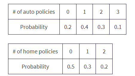
What is the expected value or mean for the overall number of policies sold per day?
Assuming the selling of new auto policies is independent of the selling of new home policies (which may not be true if some new customers buy both), what would be the standard deviation in the number of new policies sold per day?
Solution:
µauto= (0)(0.2) + (1)(0.4) + (2)(0.3) + (3)(0.1) = 1.3,
µhome= (0)(0.5) + (1)(0.3) + (2)(0.2) = 0.7, and so
µtotal = µauto + µhome = 1.3 + 0.7 = 2.0.σ2auto= (0 − 1.3)2(0.2) + (1 − 1.3)2(0.4) + (2 − 1.3)2(0.3) + (3 − 1.3)2(0.1) = 0.81,
σ2home = (0 − 0.7)2(0.5) + (1 − 0.7)2(0.3) + (2 − 0.7)2(0.2) = 0.61, and so, assuming independence, σ2total = σ2auto + σ2home = 0.81 + 0.61 = 1.42 and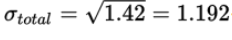
Transforming Random Variables
Adding a constant to every value of a random variable will increase the mean by that constant.
Differences between values remain the same, so measures of variability like the standard deviation will remain unchanged.
Multiplying every value of a random variable by a constant will increase the mean by the same multiple. In this case, differences are also increased and the standard deviation will increase by the same multiple.
➥ Example 4.8
A carnival game of chance has payoffs of $2 with probability 0.5, of $5 with probability 0.4, and of $10 with probability 0.1. What should you be willing to pay to play the game? Calculate the mean and standard deviation for the winnings if you play this game.
Solution:
![]()
You should be willing to pay any amount less than or equal to $4.
![]()
What if $4 is added to each payoff?
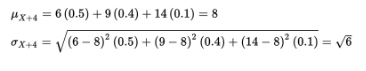
Note that µX+4 = µX + 4 and σX+4 = σX.
What if instead each payoff is tripled?
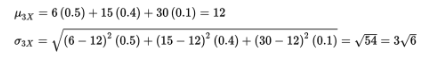
Note that µ3X = 3µX and σ3X = 3σX
Binomial Distribution
Probability distribution - is a list or formula that gives the probability of each outcome.
For applications in which a two-outcome situation is repeated a certain number of times, where each repetition is independent of the other repetitions, and in which the probability of each of the two outcomes remains the same for each repetition, the resulting calculations involve what are known as binomial probabilities.
➥ Example 4.9
Suppose the probability that a lightbulb is defective is 0.1 (so probability of being good is 0.9).
What is the probability that four lightbulbs are all defective?
What is the probability that exactly two out of three lightbulbs are defective?
What is the probability that exactly three out of eight lightbulbs are defective?
Solution:
Because of independence (i.e., whether one lightbulb is defective is not influenced by whether any other lightbulb is defective), we can multiply individual probabilities of being defective to find the probability that all the bulbs are defective:
(0.1)(0.1)(0.1)(0.1) = (0.1)4 = 0.0001
The probability that the first two bulbs are defective and the third is good is (0.1)(0.1)(0.9) = 0.009. The probability that the first bulb is good and the other two are defective is (0.9)(0.1)(0.1) = 0.009. Finally, the probability that the second bulb is good and the other two are defective is (0.1)(0.9)(0.1) = 0.009. Summing, we find that the probability that exactly two out of three bulbs are defective is 0.009 + 0.009 + 0.009 = 3(0.009) = 0.027.
The probability of any particular arrangement of three defective and five good bulbs is (0.1)3(0.9)5 = 0.00059049. We need to know the number of such arrangements.
The answer is given by combinations:
Thus, the probability that exactly three out of eight light bulbs are defective is 56 × 0.00059049 = 0.03306744. [On the TI-84, binompdf(8,0.1,3)= 0.03306744.]
Geometric Distribution
Suppose an experiment has two possible outcomes, called success and failure, with the probability of success equal to p and the probability of failure equal to q = 1 − p and the trials are independent. Then the probability that the first success is on trial number X = k is

➥ Example 4.10
Suppose only 12% of men in ancient Greece were honest. What is the probability that the first honest man Diogenes encounters will be the third man he meets? What is the probability that the first honest man he encounters will be no later than the fourth man he meets?
Solution:
This is a geometric distribution with p = 0.12. Then P(X=3) = (0.88)2(0.12) = 0.092928, where X is the number of men needed to be met in order to encounter an honest man. [Or we can calculate geometpdf (0.12, 3) = 0.092928.] This is a geometric distribution with p = 0.12. Then = geometcdf (0.12, 4) = 0.40030464. [Or we could calculate (0.12) + (0.88)(0.12) + (0.88)2(0.12) + (0.88)3(0.12) = 0.40030464.]
To receive full credit for geometric distribution probability calculations, students need to state:
Name of the distribution ("geometric" in the example above)
Parameter ("p = 0.12" in the example above)
The trial on which the first success occurs ("X = 3" in the first question above)
Correct probability (“0.092928” in the first question above)
Cumulative Probability Distribution
Probability distribution - is a function, table, or graph that links outcomes of a statistical experiment with its probability of occurrence.
Cumulative probability distribution - is a function, table, or graph that links outcomes with the probability of less than or equal to that outcome occurring.
➥ Example 4.11
The scores received on the 2019 AP Statistics exam are illustrated in the following tables:
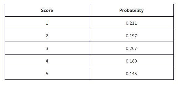
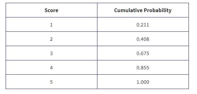
What is the probability that a student did not receive college credit (assuming you need a 3 or higher to receive college credit)?
Solution: the probability was 0.211 + 0.197 = 0.408 that a student received a 1 or 2 and thus did not receive college credit.
Unit 5: Sampling Distributions
Normal Distribution Calculations
The normal distribution - provides a valuable model for how many sample statistics vary, under repeated random sampling from a population.
Calculations involving normal distributions are often made through z**-scores**, which measure standard deviations from the mean.
On the TI-84, normalcdf(lowerbound, upperbound) gives the area (probability) between two z-scores, while invNorm(area) gives the z-score with the given area (probability) to the left. The TI-84 also has the capability of working directly with raw scores instead of z-scores. In this case, the mean and standard deviation must be given:
Normalcdf(lowerbound, upperbound, mean, standard deviation)invNorm(area, mean, standard deviation)
➥ Example 5.1
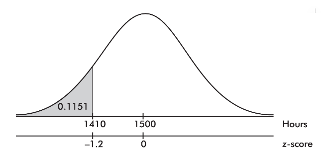
The life expectancy of a particular brand of lightbulb is roughly normally distributed with a mean of 1500 hours and a standard deviation of 75 hours.
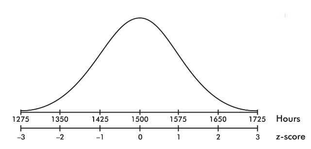
What is the probability that a lightbulb will last less than 1410 hours?
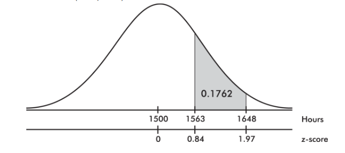
What is the probability that a lightbulb will last between 1563 and 1648 hours?
What is the probability that a lightbulb will last between 1416 and 1677 hours?
Solution:
The z-score of 1410 is
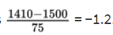
On the TI-84, normalcdf(0, 1410, 1500, 75) = 0.1151 and normalcdf(−10, −1.2) = 0.1151.
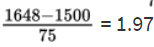
The z-score of 1563 is
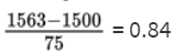
and the z-score of 1648 is
Then we calculate the probability of between 1563 and 1648 hours by normalcdf(1563, 1648, 1500, 75) = 0.1762 or normalcdf(0.84, 1.97) = 0.1760.
3. The z-score of 1416 is
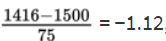
and the z-score of 1677 is
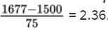
Then we calculate the probability of between 1416 and 1677 hours by normalcdf(1416, 1677, 1500, 75) = 0.8595 or normalcdf(−1.12, 2.36) = 0.8595.
To receive full credit for probability calculations using the probability distributions, you need to show:
Name of the distribution ("normal" in the example above)
Parameters ("µ = 1500, σ = 75" in the example above)
Boundary ("1410" in (a) of the example above)
Values of interest ("<" in (a) of the example above)
Correct probability (0.1151 in (a) of the example above)
Central Limit Theorem
The following principle forms the basis of much of what we discuss in this unit and in those following. Statement 1 is called the central limit theorem of statistics (often simply abbreviated as CLT)
Start with a population with a given mean µ, a standard deviation σ, and any shape distribution whatsoever. Pick n sufficiently large (at least 30), and take all samples of size n. Compute the mean of each of these samples:
the set of all sample means is approximately normally distributed (often stated: the distribution of sample means is approximately normal).
the mean of the set of sample means equals µ, the mean of the population.
the standard deviation of the set of sample means is approximately equal to, that is, to the standard deviation of the whole population divided by the square root of the sample size.
Alternatively, we say that for sufficiently large n, the sampling distribution of x̄ is approximately normal with mean µ and standard deviation.
There are six key ideas to keep in mind:
Averages vary less than individual values.
Averages based on larger samples vary less than averages based on smaller samples.
The central limit theorem (CLT) states that when the sample size is sufficiently large, the sampling distribution of the mean will be approximately normal.
The larger the sample size n, the closer the sample distribution is to the population distribution.
The larger the sample size n, the closer the sampling distribution of x̄ is to a normal distribution.
If the original population has a normal distribution, then the sampling distribution of x̄ has a normal distribution, no matter what the sample size n.
➥ Example 5.2
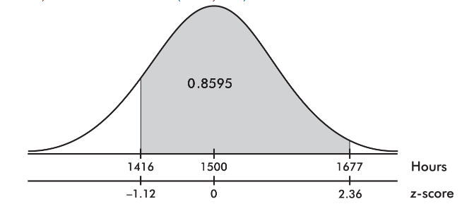
The naked mole rat, a hairless East African rodent that lives underground, has a life expectancy of 21 years with a standard deviation of 3 years. In a random sample of 40 such rats, what is the probability that the mean life expectancy is between 20 and 22 years?
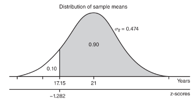
The mean life expectancy is at least how many years with a corresponding probability of 0.90?
Solution:
We have a random sample that is less than 10% of the naked mole rat population. With a sample size of n = 40 ≥ 30, the central limit theorem applies, and the sampling distribution of x̄ is approximately normal with mean
![]()
and standard deviation
![]()
The z-scores of 20 and 22 are
![]()
The probability of sample mean between 20 and 22 is normalcdf(–2.110,2.110)= 0.965. [Or normalcdf(20,22,21,0.474)= 0.965.]
The critical z-score is invNorm(0.10) = –1.282 with a corresponding raw score of 21 – 1.282(3) = 17.15 years.
Biased and Unbiased Estimators
Bias means that the sampling distribution is not centered on the population parameter.
The sampling distributions of proportions, means, and slopes are unbiased*.* That is, for a given sample size, the set of all sample proportions is centered on the population proportion, the set of all sample means is centered on the population mean, and the set of all sample slopes is centered on the population slope.
Here are some illustrative simulations:
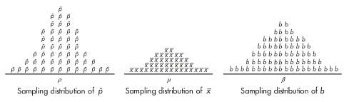
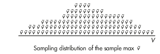
the sampling distribution for the maximum is clearly biased. That is, for a given sample size, the set of all sample maxima ṽ is not centered on the population maximum, V. For example, here is one simulation of sample maxima. Note that V falls far right of the center of the distribution of ṽ.
➥ Example 5.3
Five new estimators are being evaluated with regard to quality control in manufacturing professional baseballs of a given weight. Each estimator is tested every day for a month on samples of sizes n = 10, n = 20, and n = 40. The baseballs actually produced that month had a consistent mean weight of 146 grams. The distributions given by each estimator are as follows:
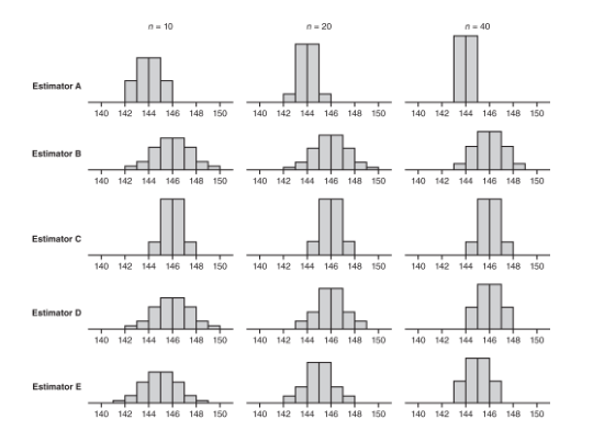
Which of the above appear to be unbiased estimators of the population parameter?
Which of the above exhibits the lowest variability for n = 40?
Which of the above is the best estimator if the selected estimator will eventually be used with a sample of size n = 100?
Solution:
Estimators B, C, and D are unbiased estimators because they appear to have means equal to the population mean of 146. A statistic used to estimate a population parameter is unbiased if the mean of the sampling distribution of the statistic is equal to the true value of the parameter being estimated.
For n = 40, estimator A exhibits the lowest variability, with a range of only 2 grams compared to the other ranges of 6 grams, 4 grams, 4 grams, and 4 grams, respectively.
Estimator D because we should choose an unbiased estimator with low variability. From part (a), we have Estimator B, C, and D as unbiased estimators. Now we look at the variability of these three statistics. As n increases, D shows tighter clustering around 146 than does B. Finally, while C looks better than D for n = 40, the estimator will be used with n = 100, and the D distribution is clearly converging as the sample size increases while the C distribution remains the same. Choose Estimator D.
Sampling Distribution for Sample Proportions
The proportion essentially represents a qualitative calculation.
The interest is simply in the presence or absence of some attribute.
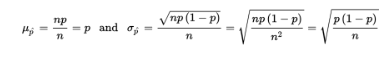
Suppose the sample size is n and the actual population proportion is p. From our work on binomial distributions, we remember that the mean and standard deviation for the number of successes in a given sample are np and √np(1-p), respectively, and for large values of n the complete distribution begins to look “normal.”
Here, however, we are interested in the proportion rather than in the number of successes. From Unit 1, remember that when we multiply or divide every element by a constant, we multiply or divide both the mean and the standard deviation by the same constant. In this case, to change number of successes to proportion of successes, we divide by n:
➥ Example 5.4
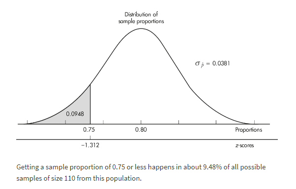
It is estimated that 80% of people with high math anxiety experience brain activity similar to that experienced under physical pain when anticipating doing a math problem. In a simple random sample of 110 people with high math anxiety, what is the probability that less than 75% experience the physical pain brain activity?
Solution:
The sample is given to be random, both np = (110)(0.80) = 88 ≥ 10 and n(1 − p) = (110)(0.20) = 22 ≥ 10, and our sample is clearly less than 10% of all people with math anxiety. So, the sampling distribution of p̂ is approximately normal with mean 0.80 and standard deviation
![]()
With a z-score of
![]()
the probability that the sample proportion is less than 0.75 is normalcdf(–1000,–1.312) = 0.0948.
[Or normalcdf(–1000, 0.75, .80, .0381) = 0.0947.]
Sampling Distribution for Differences in Sample Proportions
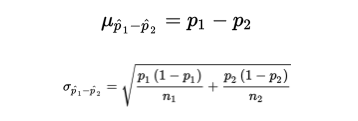
Dealing with one difference from the set of all possible differences obtained by subtracting sample proportions of one population from sample proportions of a second population.
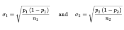
To judge the significance of one particular difference, we must first determine how the differences vary among themselves. Remember that the mean of a set of differences is the difference of the means, and the variance of a set of differences is the sum of the variances of the individual sets.
![]()
With our proportions we have
 and can calculate:
➥ Example 5.5
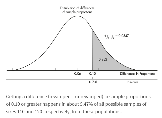
In a study of how environment affects our eating habits, scientists revamped one of two nearby fast-food restaurants with table cloths, candlelight, and soft music. They then noted that at the revamped restaurant, customers ate more slowly and 25% left at least 100 calories of food on their plates. At the unrevamped restaurant, customers tended to quickly eat their food and only 19% left at least 100 calories of food on their plates. In a random sample of 110 customers at the revamped restaurant and an independent random sample of 120 customers at the unrevamped restaurant, what is the probability that the difference in the percentages of customers in the revamped setting and the unrevamped setting is more than 10% (where the difference is the revamped restaurant percent minus the unrevamped restaurant percent)?
Solution: We have independent random samples, each less than 10% of all fast-food customers, and we note that n1p1 = 110(0.25) = 27.5, n1(1 − p1) = 110(0.75) = 82.5, n2p2 = 120(0.19) = 22.8, and n2(1 − p2) = 120(0.81) = 97.2 are all ≥10. Thus, the sampling distribution of p̂1- p̂2 is roughly normal with mean
![]()
and standard deviation
![]()
The z-score of 0.10 is
![]() , and normalcdf(0.731,1000)= 0.232. [Or normalcdf(0.10,1.0,0.06,0.0547)= 0.232.]
, and normalcdf(0.731,1000)= 0.232. [Or normalcdf(0.10,1.0,0.06,0.0547)= 0.232.]
Sampling Distribution for Sample Means
Suppose the variance of the population is σ2 and we are interested in samples of size n. Sample means are obtained by first summing together n elements and then dividing by n.
A set of sums has a variance equal to the sum of the variances associated with the original sets. In our case,
![]() When each element of a set is divided by some constant, the new variance is the old one divided by the square of the constant. Since the sample means are obtained by dividing the sums by n, the variance of the sample means is obtained by dividing the variance of the sums by n2. Thus, if σx̄ symbolizes the standard deviation of the sample means, we find that:
When each element of a set is divided by some constant, the new variance is the old one divided by the square of the constant. Since the sample means are obtained by dividing the sums by n, the variance of the sample means is obtained by dividing the variance of the sums by n2. Thus, if σx̄ symbolizes the standard deviation of the sample means, we find that:
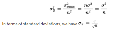
➥ Example 5.6
The number of emergency room visits after drinking energy drinks is skyrocketing. One particular energy drink has an average of 200 mg of caffeine with a standard deviation of 10 mg. A store sells boxes of six bottles each. What is the mean and standard deviation of the average milligrams of caffeine consumers should expect from the six bottles in each box?
Solution: We have samples of size 6, and 6 is assumed to be less than 10% of all such bottles. The mean of these sample means will equal the population mean of 200 mg. The standard deviation of these sample means will equal
![]() For all random samples of size n = 6 from this population, the sample mean milligrams of caffeine will have a mean of 200 mg and will typically vary by about 4.08 mg from the population mean of 200 mg.
For all random samples of size n = 6 from this population, the sample mean milligrams of caffeine will have a mean of 200 mg and will typically vary by about 4.08 mg from the population mean of 200 mg.
Sampling Distribution for Differences in Sample Means
To judge the significance of one particular difference, we must first determine how the differences vary among themselves.
The necessary key is the fact that the variance of a set of differences is equal to the sum of the variances of the individual sets. Thus:
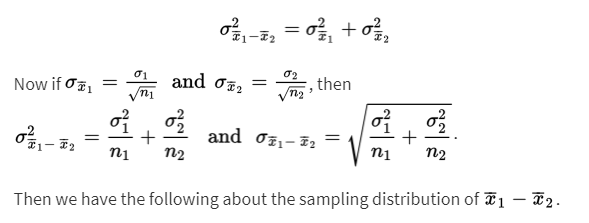
➥ Example 5.7
It is estimated that 40-year-old men contribute an average of 65 genetic mutations to their new children, whereas 20-year-old men contribute an average of only 25. Assuming standard deviations of 15 and 5 mutations, respectively, for the 40- and 20-year-olds, what is the probability that the mean number of mutations in a random sample of thirty-five 40-year-old new fathers is between 35 and 45 more than the mean number in a random sample of forty 20-year-old new fathers?
Solution: We have independent random samples, each less than 10% of their age groups, and both sample sizes are over 30, so the sampling distribution of x̄1-x̄2 is roughly normal with mean
![]() and standard deviation
and standard deviation ![]() The z-scores of 35 and 45 are
The z-scores of 35 and 45 are ![]() , respectively, and normalcdf(-1.883,1.883)= 0.940. [Or normalcdf(35,45,40,2.656)= 0.940.]
, respectively, and normalcdf(-1.883,1.883)= 0.940. [Or normalcdf(35,45,40,2.656)= 0.940.]
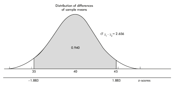
Simulation of a Sampling Distribution
The normal distribution can handle sampling distributions of the statistics we are most interested in, namely the sample proportion and sample mean.
If other statistics arise, we can use simulation to obtain a rough idea of the corresponding sampling distributions.
For example, a study is made of the number of dreams high school students remember having every night. The median number is 3.41 with a variance of 1.46 and a minimum of 0. Now taking a large number of random samples of 15 students, we calculate the median, variance, and minimum for each sample and graph the resulting simulated sampling distributions.
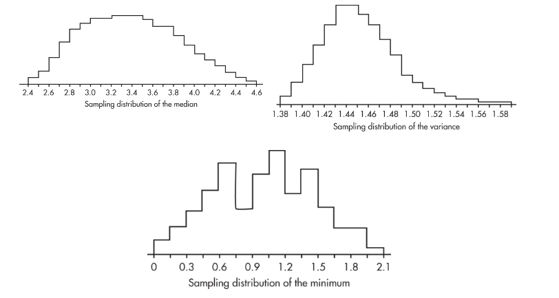
The simulated sampling distribution of these medians is roughly bell-shaped, the simulated sampling distribution of the variances is skewed right, and the simulated sampling distribution of the minimums is very roughly bell-shaped.
Unit 6: Inference for Categorical Data: Proportions
The Meaning of a Confidence Interval
The percentage is the percentage of samples that would pinpoint the unknown p or µ within plus or minus respective margins of error.
For a given sample proportion or mean, p or µ either is or isn’t within the specified interval, and so the probability is either 1 or 0.
Two aspects to this concept:
First, there is the confidence interval, usually expressed in the form:
![]()
Second, there is the success rate for the method, called the confidence level, that is, the proportion of times repeated applications of this method would capture the true population parameter.
The standard error is a measure of how far the sample statistic typically varies from the population parameter.
The margin of error is a multiple of the standard error, with that multiple determined by how confident we wish to be of our procedure.
All of the above assume that certain conditions are met. For inference on population proportions, means, and slopes, we must check for independence in data collection methods and for selection of the appropriate sampling distribution.
Conditions for Inference
The following are the two standard assumptions for our inference procedures and the "ideal" way they are met:
Independence assumption:
Individuals in a sample or an experiment an must be independent of each other, and this is obtained through random sampling or random selection.
Independence across samples is obtained by selecting two (or more) separate random samples.
Always examine how the data were collected to check if the assumption of independence is reasonable.
Sample size can also affect independence. Because sampling is usually done without replacement, if the sample is too large, lack of independence becomes a concern.
So, we typically require that the sample size n be no larger than 10% of the population (the 10% Rule).
Normality assumption:
Inference for proportions is based on a normal model for the sampling distribution of p̂, but actually we have a binomial distribution.
Fortunately, the binomial is approximately normal if both np and nq ≥ 10.
Inference for means is based on a normal model for the sampling distribution of x̄; this is true if the population is normal and is approximately true (thanks to the CLT) if the sample size is large enough (typically we accept n ≥ 30).
With regard to means, this is referred to as the Normal/Large Sample condition.
➥ Example 6.1
If we pick a simple random sample of size 80 from a large population, which of the following values of the population proportion p would allow use of the normal model for the sampling distribution of p̂?
0.10
0.15
0.90
0.95
0.99
Solution: (B)
The relevant condition is that both np and nq ≥ 10.
In (A), np = (80)(0.10) = 8; in (C), nq = (80)(0.10) = 8; in (D), nq = (80)(0.05) = 4; and in (E), nq = (80)(0.01) = 0.8. However, in (B), np = (80)(0.15) = 12 and nq = (0.85)(80) = 68 are both ≥ 10.
Confidence Interval for a Proportion
Estimating a population proportion p by considering a single sample proportion p̂.
This sample proportion is just one of a whole universe of sample proportions, and from Unit 5 we remember the following:
The set of all sample proportions is approximately normally distributed.
The mean μp̂ of the set of sample proportions equals p, the population proportion.
The standard deviation σp̂ of the set of sample proportions is approximately equal to

In finding confidence interval estimates of the population proportion p, how do we find
since p is unknown? The reasonable procedure is to use the sample proportion p̂:
When the standard deviation is estimated in this way (using the sample), we use the term standard error:
 ➥ Example 6.2
If 42% of a simple random sample of 550 young adults say that whoever asks for the date should pay for the first date, determine a 99% confidence interval estimate for the true proportion of all young adults who would say that whoever asks for the date should pay for the first date.
Does this confidence interval give convincing evidence in support of the claim that fewer than 50% of young adults would say that whoever asks for the date should pay for the first date?
Solution:
The parameter is p, which represents the proportion of the population of young adults who would say that whoever asks for the date should pay for the first date. We check that
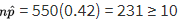
![]()
We are given that the sample is an SRS, and 550 is clearly less than 10% of all young adults. Since p̂ = 0.42, the standard error of the set of sample proportions is
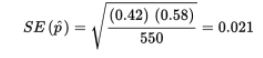
99% of the sample proportions should be within 2.576 standard deviations of the population proportion. Equivalently, we are 99% certain that the population proportion is within 2.576 standard deviations of any sample proportion.
Thus, the 99% confidence interval estimate for the population proportion is 0.42 ± 2.576(0.021) = 0.42 ± 0.054. We say that the margin of error is ±0.054. We are 99% confident that the true proportion of young adults who would say that whoever asks for the date should pay for the first date is between 0.366 and 0.474.
Yes, because all the values in the confidence interval (0.366 to 0.474) are less than 0.50, this confidence interval gives convincing evidence in support of the claim that fewer than 50% of young adults would say that whoever asks for the date should pay for the first date.
Logic of Significance Testing
Closely related to the problem of estimating a population proportion or mean is the problem of testing a hypothesis about a population proportion or mean.
The general testing procedure is to choose a specific hypothesis to be tested, called the null hypothesis, pick an appropriate random sample, and then use measurements from the sample to determine the likelihood of the null hypothesis.
If the sample statistic is far enough away from the claimed population parameter, we say that there is sufficient evidence to reject the null hypothesis. We attempt to show that the null hypothesis is unacceptable by showing that it is improbable.
The null hypothesis H0 is stated in the form of an equality statement about the population proportion (for example, H0: p = 0.37).
There is an alternative hypothesis, stated in the form of a strict inequality (for example, Ha: p < 0.37 or Ha: p > 0.37 or Ha: p ≠ 0.37).
The strength of the sample statistic p̂ can be gauged through its associated P-value, which is the probability of obtaining a sample statistic as extreme (or more extreme) as the one obtained if the null hypothesis is assumed to be true. The smaller the P-value, the more significant the difference between the null hypothesis and the sample results.
There are two types of possible errors:
the error of mistakenly rejecting a true null hypothesis.
the error of mistakenly failing to reject a false null hypothesis.
The α-risk, also called the significance level of the test, is the probability of committing a Type I error and mistakenly rejecting a true null hypothesis.
Type II error - a mistaken failure to reject a false null hypothesis, has associated probability β.
There is a different value of β for each possible correct value for the population parameter p. For each β, 1 − β is called the "power" of the test against the associated correct value.
Power of a hypothesis test - is the probability that a Type II error is not committed.
That is, given a true alternative, the power is the probability of rejecting the false null hypothesis. Increasing the sample size and increasing the significance level are both ways of increasing the power. Also note that a true null that is further away from the hypothesized null is more likely to be detected, thus offering a more powerful test.
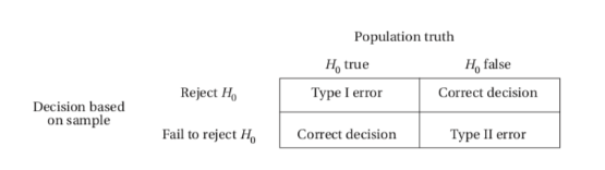
A simple illustration of the difference between a Type I and a Type II error is as follows.
Suppose the null hypothesis is that all systems are operating satisfactorily with regard to a NASA launch. A Type I error would be to delay the launch mistakenly thinking that something was malfunctioning when everything was actually OK. A Type II error would be to fail to delay the launch mistakenly thinking everything was OK when something was actually malfunctioning. The power is the probability of recognizing a particular malfunction. (Note the complementary aspect of power, a “good” thing, with Type II error, a “bad” thing.)
It should be emphasized that with regard to calculations, questions like “What is the power of this test?” and “What is the probability of a Type II error in this test?” cannot be answered without reference to a specific alternative hypothesis.
Significance Test for a Proportion
It is important to understand that because the P-value is a conditional probability, calculated based on the assumption that the null hypothesis, H0: p = p0, is true, we use the claimed proportion p0 both in checking the np0 ≥ 10 and n(1 − p0) ≥ 10 conditions and in calculating the standard deviation
![]()
➥ Example 6.3
A union spokesperson claims that 75% of union members will support a strike if their basic demands are not met. A company negotiator believes the true percentage is lower and runs a hypothesis test. What is the conclusion if 87 out of a simple random sample of 125 union members say they will strike?
For each of the two possible answers above, what error might have been committed, Type I or Type II, and what would be a possible consequence?
Solution:
Parameter: Let p represent the proportion of all union members who will support a strike if their basic demands are not met.
Hypotheses: H0: p = 0.75 and Ha: p < 0.75.
Procedure: One-sample z-test for a population proportion.
Checks: np0 = (125)(0.75) = 93.75 and n(1 − p0) = (125)(0.25) = 31.25 are both ≥ 10, it is given that we have an SRS, and we must assume that 125 is less than 10% of the total union membership.
Mechanics: Calculator software (such as 1-PropZTest on the TI-84 or Z-1-PROP on the Casio Prizm) gives z = −1.394 and P = 0.0816.
Conclusion in context with linkage to the P-value: There are two possible answers:
a. With this large of a P-value, 0.0816 > 0.05, there is not sufficient evidence to reject H0; that is, there is not sufficient evidence at the 5% significance level that the true percentage of union members who support a strike is less than 75%.
b. With this small of a P-value, 0.0816 < 0.10, there is sufficient evidence to reject H0; that is, there is sufficient evidence at the 10% significance level that the true percentage of union members who support a strike is less than 75%.
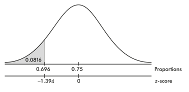
If the P-value is considered large, 0.0816 > 0.05, so that there is not sufficient evidence to reject the null hypothesis, there is the possibility that a false null hypothesis would mistakenly not be rejected and thus a Type II error would be committed. In this case, the union might call a strike thinking they have greater support than they actually do. If the P-value is considered small, 0.0816 < 0.10, so that there is sufficient evidence to reject the null hypothesis, there is the possibility that a true null hypothesis would mistakenly be rejected, and thus a Type I error would be committed. In this case, the union might not call for a strike thinking they don’t have sufficient support when they actually do have support.
Confidence Interval for the Difference of Two Proportions
From Unit 5, we have the following information about the sampling distribution of
![]()
The set of all differences of sample proportions is approximately normally distributed.
The mean of the set of differences of sample proportions equals p1 − p2, the difference of the population proportions.
The standard deviation
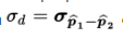
of the set of differences of sample proportions is approximately equal to:
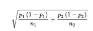
Remember that we are using the normal approximation to the binomial, so
![]()
should all be at least 10. In making calculations and drawing conclusions from specific samples, it is important both that the samples be simple random samples and that they be taken independentlyof each other. Finally, the original populations should be large compared to the sample sizes, that is, check that
![]()
➥ Example 6.4
Suppose that 84% of a simple random sample of 125 nurses working 7:00 a.m. to 3:00 p.m. shifts in city hospitals express positive job satisfaction, while only 72% of an SRS of 150 nurses on 11:00 p.m. to 7:00 a.m. shifts express similar fulfillment. Establish a 90% confidence interval estimate for the difference.
Based on the interval, is there convincing evidence that the nurses on the 7 AM to 3 PM shift express a higher job satisfaction than nurses on the 11 PM to 7 AM shift?
Solution:
Parameters: Let p1 represent the proportion of the population of nurses working 7:00 a.m. to 3:00 p.m. shifts in city hospitals who have positive job satisfaction. Let p2 represent the proportion of the population of nurses working 11:00 p.m. to 7:00 a.m. shifts in city hospitals who have positive job satisfaction.
Procedure: Two-sample z-interval for a difference between population proportions, p1 − p2.
Checks:
![]()
![]()
we are given independent SRSs; and the sample sizes are assumed to be less than 10% of the populations of city hospital nurses on the two shifts, respectively.
Mechanics: 2-PropZInt on the TI-84 or 2-Prop ZInterval on the Casio Prizm give (0.0391, 0.2009).
The observed difference is 0.84 − 0.72 = 0.12, and the critical z-scores are ±1.645. The confidence interval estimate is 0.12 ± 1.645(0.0492) = 0.12 ± 0.081.]
Conclusion in context: We are 90% confident that the true proportion of satisfied nurses on 7:00 a.m. to 3:00 p.m. shifts is between 0.039 and 0.201 higher than the true proportion for nurses on 11:00 p.m. to 7:00 a.m. shifts.
Yes, because the entire interval from 0.039 to 0.201 is positive, there is convincing evidence that the nurses on the 7 AM to 3 PM shift express a higher job satisfaction than nurses on the 11 PM to 7 AM shift.
Significance Test for the Difference of Two Proportions
The null hypothesis for a difference between two proportions is
![]()
and so the normality condition becomes that
![]()
![]() should all be at least 10, where p̂ is the combined (or pooled) proportion,
should all be at least 10, where p̂ is the combined (or pooled) proportion, ![]() The other important conditions to be checked are both that the samples be random samples, ideally simple random samples, and that they be taken independently of each other. The original populations should also be large compared to the sample sizes, that is, check that
The other important conditions to be checked are both that the samples be random samples, ideally simple random samples, and that they be taken independently of each other. The original populations should also be large compared to the sample sizes, that is, check that
![]()
Two points need to be stressed:
First, sample proportions from the same population can vary from each other.
Second, what we are really comparing are confidence interval estimates, not just single points.
For many problems, the null hypothesis states that the population proportions are equal or, equivalently, that their difference is 0:
![]()
The alternative hypothesis is then:
![]()
where the first two possibilities lead to one-sided tests and the third possibility leads to a two-sided test.
Since the null hypothesis is that p1 = p2, we call this common value pc and use this pooled value in calculating σd:
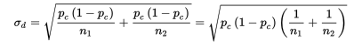
In practice, if
![]()
we use
![]()
as an estimate of pc in calculating σd.
➥ Example 6.5
In a random sample of 1500 First Nations children in Canada, 162 were in child welfare care, while in an independent random sample of 1600 non-Aboriginal children, 23 were in child welfare care. Many people believe that the large proportion of indigenous children in government care is a humanitarian crisis. Do the above data give significant evidence that a greater proportion of First Nations children in Canada are in child welfare care than the proportion of non-Aboriginal children in child welfare care?
Does a 95% confidence interval for the difference in proportions give a result consistent with the above conclusion?
Solution:
Parameters: Let p1 represent the proportion of the population of First Nations children in Canada who are in child welfare care. Let p2 represent the proportion of the population of non-Aboriginal children in Canada who are in child welfare care.
Hypotheses: H0: p1 − p2 = 0 or H0: p1 = p2 and Ha: p1 – p2 > 0 or Ha: p1 > p2.
Procedure: Two-sample z-test for a difference of two population proportions.
Checks:
![]()
![]()
are all at least 10; the samples are random and independent by design; and it is reasonable to assume the sample sizes are less than 10% of the populations.
Mechanics: Calculator software (such as 2-PropZTest) gives z = 11.0 and P = 0.000.
Conclusion in context with linkage to the P-value: With this small of a P-value, 0.000 < 0.05, there is sufficient evidence to reject H0; that is, there is convincing evidence that that the true proportion of all First Nations children in Canada in child welfare care is greater than the true proportion of all non-Aboriginal children in Canada in child welfare care.
Calculator software (such as 2-PropZInt) gives that we are 95% confident that the true difference in proportions (true proportion of all First Nations children in Canada in child welfare care minus the true proportion of all non-Aboriginal children in Canada in child welfare care) is between 0.077 and 0.110. Since this interval is entirely positive, it is consistent with the conclusion from the hypothesis test.
Unit 7: Inference for Quantitative Data: Means
The t-distribution
When the population standard deviation σ is unknown, we use the sample standard deviation s as an estimate for σ.
This Student’s t-distribution - was introduced in 1908 by W. S. Gosset, a British mathematician employed by the Guinness Breweries.
For a sample from a normally distributed population, we work with the variable

with a resulting t-distribution that is bell-shaped and symmetric but lower at the mean, higher at the tails, and so more spread out than the normal distribution.
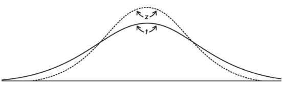
The t-distribution is different for different values of n.
In the tables, these distinct t-distributions are associated with the values for degrees of freedom (df).
For this discussion, the df value is equal to the sample size minus 1. The smaller the df value, the larger the dispersion in the distribution. The larger the df value, that is, the larger the sample size, the closer the distribution to the normal distribution.
Thus, the t-distribution is the proper choice whenever the population standard deviation σ is unknown.
In the real world, σ is almost always unknown, and so we should almost always use the t-distribution.
Confidence Interval for a Mean
This sample mean is just one of a whole universe of sample means, and we remember that if n is sufficiently large:
the set of all sample means is approximately normally distributed.
the mean of the set of sample means equals µ, the mean of the population.
the standard deviation
 of the set of sample means is approximately equal to
  , that is, equal to the standard deviation of the whole population divided by the square root of the sample size.
Typically we do not know σ, the population standard deviation. In such cases, we must use s, the standard deviation of the sample, as an estimate of σ.
In this case

is called the standard error
![]()
, and is used as an estimate for
![]()
➥ Example 7.1
When a random sample of 10 cars of a new model was tested for gas mileage, the results showed a mean of 27.2 miles per gallon with a standard deviation of 1.8 miles per gallon.
What is a 95% confidence interval estimate for the mean gas mileage achieved by this model? (Assume that the population of mpg results for all the new model cars is approximately normally distributed.)
Based on this confidence interval, do you think that the true mean mileage is significantly different from 25 mpg?
Determine a 99% confidence interval.
What would the 95% confidence interval be if the sample mean of 27.2 and standard deviation of 1.8 had come from a sample of 20 cars?
With the original data
![]()
, with what confidence can we assert that the true mean gas mileage is 27.2 ± 1.04?
Solution:
Parameter: Let μ represent the mean gas mileage (in miles per gallon) in the population of cars of a new model.
Procedure: A one-sample t-interval for a population mean.
Checks: The sample is given to be random, 10 cars are assumed to be less than 10% of all cars of the new model, and the population is stated to be approximately normal. So,
![]()
follows a t-distribution.
Mechanics: Calculator software (such as TInterval on the TI-84 or 1-Sample tInterval on the Casio Prizm) gives (25.912, 28.488).
Conclusion in context: We are 95% confident that the true mean gas mileage of all cars of the new model is between 25.91 and 28.49 miles per gallon.
Yes, because 25 is not in the interval of plausible values from 25.9 to 28.5, there is convincing evidence that the true mean mileage is significantly different from 25 mpg.
Here, TInterval gives (25.35, 29.05). We are 99% confident that the true mean gas mileage of all cars of the new model is between 25.35 and 29.05 miles per gallon. Note that when we want a higher confidence (99% instead of 95%), we have to settle for a larger, less specific interval (±1.85) instead of (±1.29).
Here, TInterval gives (26.36, 28.04). We are 95% confident that the true mean gas mileage of all cars of the new model is between 26.36 and 28.04 miles per gallon. Note that when the sample size increased (from n = 10 to n = 20), the same sample mean and standard deviation resulted in a narrower, more specific interval (±0.84) instead of (±1.29).
Converting ±1.04 to t-scores yields
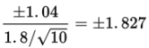
and tcdf(-1.827, 1.827, 9) = 0.899 = 89.9%. We are 89.9% confident that the true mean gas mileage of all cars of the new model is between 26.16 and 28.24 miles per gallon.
Significance Test for a Mean
To conduct a significance test for a mean, we must check that we have a simple random sample, that the sample size is less than 10% of the population, and that either the sample size is large enough (n ≥ 30) for the CLT to apply or the population has an approximately normal distribution (either stated or if we are given the sample data, a plot should be unimodal and reasonably symmetric, showing no outliers and no skewness).
➥ Example 7.2
A manufacturer claims that a new brand of air-conditioning units uses only 6.5 kilowatts of electricity per day. A consumer agency believes the true figure is higher and runs a test on a random sample of size 50. If the sample mean is 7.0 kilowatts with a standard deviation of 1.4, should the manufacturer’s claim be rejected at a significance level of 5%? Of 1%?
Given the above conclusion, what type of error, Type-I or Type-II, might have been committed, and what would be a possible consequence?
Solution:
Parameter: Let μ represent the mean electricity usage (in kilowatts per day) of the population of a new brand of air-conditioning unit.
Hypotheses: H0: μ = 6.5 and Ha: μ > 6.5.
Procedure: A one-sample t-test for a population mean (population SD is unknown).
Checks: We are given a random sample, n = 50 ≥ 30 is large enough for the CLT to apply, and we can assume that 50 is less than 10% of all of the new AC units.
Mechanics: Calculator software (such as T-Test on the TI-84) gives t = 2.525 and P = 0.0074.
Conclusion in context with linkage to the P-value: With this small of a P-value, 0.0074 < 0.05, there is convincing evidence to reject H0; that is, there is sufficient evidence for the consumer agency to reject the manufacturer’s claim that the new unit uses a mean of only 6.5 kilowatts of electricity per day.
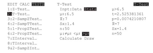
There was sufficient evidence to reject the null hypothesis. If the null hypothesis were true, we would be committing a Type-I error, that is, mistakenly rejecting a true null hypothesis. A possible consequence here is that the consumer agency would discourage customers from purchasing a new brand of air-conditioning unit that really was saving on electricity consumption as advertised.
Confidence Interval for the Difference of Two Means
We have the following information about the sampling distribution of
![]()
The set of all differences of sample means is approximately normally distributed.
The mean of the set of differences of sample means equals µ1 – µ2, the difference of population means.
The standard deviation
![]()
of the set of differences of sample means is approximately equal to
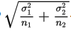
When the population standard deviations are unknown, use a t-distribution with
. There is the additional condition that either the original populations are roughly normal or the sample sizes are large enough (n1 ≥ 30 and n2 ≥ 30) for the CLT to apply.
➥ Example 7.3
A 30-month study is conducted to determine the difference in the numbers of accidents per month occurring in two departments in an assembly plant. Suppose the first department averages 12.3 accidents per month with a standard deviation of 3.5, while the second averages 7.6 accidents with a standard deviation of 3.4. Determine a 95% confidence interval estimate for the mean difference in the numbers of accidents per month. (Assume that the two populations are independent and approximately normally distributed.)
Based on this confidence interval, do you think that there is a significant mean difference (first department minus second department) in accidents per month between the two departments?
Solution:
Parameters: Let μ1 represent the mean number of accidents in the population of the number of accidents in all months for the first department. Let μ2 represent the mean number of accidents in the population of the number of accidents in all months for the second department.
Procedure: A two-sample t-interval for a difference between two population means (first department minus second department).
Checks: We are not given that the sample is random, so we must assume that the 30 months are representative. We are given that the two populations are independent and approximately normal, so a t-interval may be found (population SDs are unknown).
Mechanics: Calculator software (such as 2-SampTInt on the TI-84 or 2-Sample tInterval on the Casio Prizm) gives (2.9167, 6.4833).
Conclusion in context: We are 95% confident that the first department has a true mean of between 2.92 and 6.48 more accidents per month than the second department.
Yes, because the entire interval from 2.92 to 6.48 is positive, there is convincing evidence that the mean difference in accidents per month between the two departments is significant.
Significance Test for the Difference of Two Means
A Significance test for the difference of two means requires us to check that we have two independent simple random samples and that either the original two populations are roughly normal or the sample sizes are each large enough (n1 ≥ 30 and n2 ≥ 30) for the CLT to apply.
In this situation, the null hypothesis is usually that the means of the populations are the same or, equivalently, that their difference is 0:
![]()
The alternative hypothesis is then:
![]()
The first two possibilities lead to one-sided tests, and the third possibility leads to two-sided tests.
➥ Example 7.4
A sales representative believes that the computer his company sells has more average non-operational time per week than a similar model of computer sold by a competitor. Before taking this concern to his director, the sales representative gathers data and runs a significance test. He determines that in a simple random sample of 40 week-long periods at different firms using his company’s product, the average downtime was 125 minutes per week with a standard deviation of 37 minutes. However, 35 week-long periods involving the competitor’s computer yield an average downtime of only 115 minutes per week with a standard deviation of 43 minutes. What conclusion should the sales representative draw?
Given the above conclusion, what type of error, Type-I or Type-II, might have been committed, and what would be a possible consequence?
Solution:
Parameters: Let μ1 represent the mean of the population of non-operational times of the company's model computer. Let μ2 represent the mean of the population of non-operational times of the competitor's model computer.
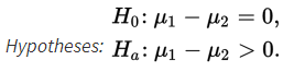
Procedure: A two-sample t-test for the difference of two population means.
Checks: We are given independent SRSs, and the sample sizes are large enough (n1 = 40 ≥ 30 and n2 = 35 ≥ 30) for the CLT to apply. The population SDs are unknown, so a t-test is appropriate.
Mechanics: Calculator software gives t = 1.0718 and P = 0.1438.
Conclusion in context with linkage to the P-value: With this large of a P-value, 0.1438 > 0.05, there is not convincing evidence to reject H0; that is, the sales representative does not have convincing evidence that his company’s computers have greater mean non-operational time than that of the competitor’s computers.
There was not sufficient evidence to reject the null hypothesis. If the null hypothesis were false, we would be committing a Type-II error, that is, mistakenly failing to reject a false null hypothesis. A possible consequence here is that the company’s computers do have a greater mean non-operational time than those of the competitor’s, but because the test doesn’t show this, the company doesn’t make necessary fixes and future sales will suffer.
Paired Data
When we have a quantitative variable measured twice for the same individual or for two very similar individuals, inference on the true mean difference involves one-sample analysis on the single variable consisting of the differences from the paired data.
➥ Example 7.5
An SAT preparation class of 30 randomly selected students produces the following total score summary:
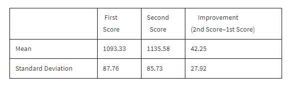
Find a 90% confidence interval of the mean improvement in test scores.
Solution: It would be wrong to calculate a confidence interval for a difference between two means using the means and standard deviations of the first and second scores. The independence condition between the two samples is violated! The proper procedure is a one-sample t-interval on the set of differences (improvement) between the scores for each of the 30 students.
Parameter: Let μ represent the mean improvement (2nd score minus 1st score) in the SAT scores of the population of students who take this SAT preparation class.
Procedure: A one-sample t-interval for the mean of a population of differences in paired data.
Checks: We are given a random sample, n = 30 is less than 10% of all students, and n = 30 is large enough so that the CLT applies.
Mechanics: With an unknown population SD, it's necessary to find a t-interval. Using X̄ = 42.25 and s = 27.92, calculator software (such as TInterval) gives (33.59, 50.91).
Conclusion in context: We are 90% confident that the true mean improvement in test scores is between 33.59 and 50.91.
Simulations and P-Values
We can use a simulation to determine what values of a test statistic are likely to occur by random chance alone, assuming the null hypothesis is true.
Then looking at where our test statistic falls, we can estimate a P**-value**.
➥ Example 7.6
One measure of variability is the median absolute deviation (MAD). It is defined as the median deviation from the median, that is, as the median of the absolute values of the deviations from the median. A particular industrial product has the following quality control check. Random samples of size 6 are gathered periodically, and measurements are taken of the dimension under observation. If the MAD calculation is significantly greater than what is expected during proper operation of the machinery, a recalibration is necessary. In a simulation of 100 such samples of size 6 from when the machinery is working properly, the resulting MAD calculations are summarized in the following dotplot:
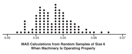
Suppose in a random sample of 6 products the measurements are {8.04, 8.06, 8.10, 8.14, 8.18, 8.19}. Is there sufficient evidence to necessitate a recalibration of the machinery?
Solution: The median is
![]()
. The absolute deviations from the median are {0.08, 0.06, 0.02, 0.02, 0.06, 0.07} with median
![]()
(the MAD calculation). In the simulation, there were 3 values out of 100 that were 0.06 or greater. This gives an estimated P-value of 0.03. With this small of a P-value, 0.03 < 0.05, there is sufficient evidence to necessitate a recalibration of the machinery.
More on Power, Type I Errors, and Type II Errors
Type II error - is a mistaken failure to reject the false null hypothesis, while the power is the probability of rejecting that false null hypothesis.
➥ Example 7.7
A candidate claims to have the support of 70% of the people, but you believe that the true figure is lower. You plan to gather an SRS and will reject the 70% claim if your sample shows 65% or less support. What if, in reality, only 63% of the people support the candidate?
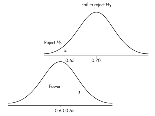
The upper graph shows the null hypothesis model with the claim that p0 = 0.70 and the plan to reject H0 if
![]()
The lower graph shows the true model with p = 0.63. When will we fail to recognize that the null hypothesis is incorrect? Answer: precisely when the sample proportion is greater than 0.65. This is a Type II error with probability β. When will we rightly conclude that the null hypothesis is incorrect? Answer: when the sample proportion is less than 0.65. This is the "power" of the test and has probability 1 − β.
Confidence Intervals Versus Hypothesis Tests
A claim about a population parameter indicates a hypothesis test, while an estimate of a population parameter asks for a confidence interval.
➥ Example 7.8
Suppose it is reported that random samples of 3-point shots by basketball players Stephen Curry and Michael Jordan show a 43% rate for Curry and a 33% rate for Jordan.
(a) Are these numbers parameters or statistics?
(b) State appropriate hypotheses for testing whether the difference is statistically significant.
(c) Suppose the sample sizes were both 100. Find the z-statistic and the P-value, and give an appropriate conclusion at the 5% significance level.
(d) Calculate and interpret a 95% confidence interval for the difference in population proportions.
(e) Are the test decision and confidence interval consistent with each other?
(f) Repeat (c), (d), and (e) as if the sample size had been 200 for each.
Solutions:
(a) These two numbers are statistics because they describe samples, not all 3-point shots ever taken by these two players.
(b) H0: pCurry = pJordan and Ha: pCurry ≠ pJordan.
(c) Calculator software gives z = 1.46 and P = 0.145. With this large of a P-value, 0.145 > 0.05, there is not sufficient evidence to reject H0; that is, there is not convincing evidence of a difference in the true 3-point percentage rates of Curry and Jordan.
(d) Calculator software gives (−0.034, 0.234). We are 95% confident that the true difference in 3-point percentage rates (Curry minus Jordan) is between −3.4% and 23.4%.
(e) Yes, they are consistent. We did not conclude that the two percentages differ, and the confidence interval (for the difference in population proportions) includes the value zero.
(f) With a sample size of 200, calculator software gives z = 2.06 and P = 0.039. With this small a P-value, 0.039 < 0.05, there is sufficient evidence to reject H0; that is, there is convincing evidence of a difference in the true 3-point percentage rates of Curry and Jordan. With a sample size of 200, calculator software gives a confidence interval of (0.005, 0.195). We are 95% confident that the true difference in 3-point percentage rates (Curry minus Jordan) is between 0.5% and 19.5%. This interval does not include zero, so it is convincing evidence of a difference in the true 3-point percentage rates of Curry and Jordan. This is again consistent with the hypothesis test.
Unit: 8 Inference for Categorical Data: Chi-Square
Chi-Square Test for Goodness-of-Fit
A perfect fit cannot be expected, and so we must look at discrepancies and make judgments as to the Goodness-of-fit.
There is the null hypothesis of a good fit, that is, the hypothesis that a given theoretical distribution correctly describes the situation, problem, or activity under consideration.
The sum of these weighted differences or discrepancies is called the chi-square statistic and is denoted as χ2 (χ is the lowercase Greek letter chi):
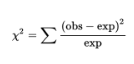
The smaller the resulting χ2-value, the better the fit.
The P**-value** is the probability of obtaining a χ2-value as extreme as (or as more extreme than) the one obtained if the null hypothesis is assumed true.
If the χ2-value is large enough, that is, if the P-value is small enough, we say there is sufficient evidence to reject the null hypothesis and to claim that the fit is poor.
To decide how large a calculated χ2-value must be to be significant, that is, to choose a critical value, we must understand how χ2-values are distributed.
A χ2-distribution has only nonnegative values, is not symmetric, and is always skewed to the right.
There are distinct χ2-distributions, each with an associated number of degrees of freedom (df).
The larger the df value, the less pronounced is the skew, and the closer the χ2-distribution is to a normal distribution.
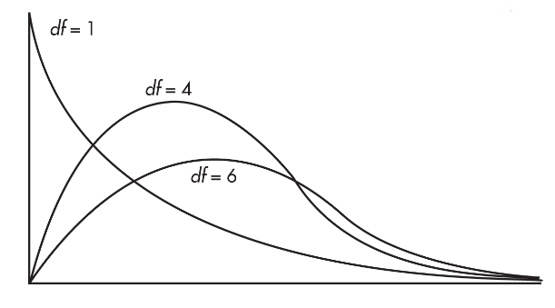
For inference about the distribution of a single categorical variable, such as a goodness-of-fit test, we will use a chi-square distribution with degrees of freedom, df = number of categories - 1.
➥ Example 8.1
A large city is divided into four distinct socioeconomic regions, one where the upper class lives, one for the middle class, one for the lower class, and one mixed-class region. Area percentages of the regions are 12%, 38%, 32%, and 18%, respectively. In a random sample of 55 liquor stores in the city, the numbers from each region are 4, 16, 26, and 9, respectively. The following shows how to determine if there is statistical evidence that region makes a difference with regard to numbers of liquor stores.
If liquor stores in the city were distributed among the four regions in the same proportions as the areas of those regions, what number (out of 55) would be expected in each region?
Are the sample numbers 4, 16, 26, and 9 significantly different from the expected values 6.6, 20.9, 17.6, and 9.9 to indicate that region makes a difference with regard to numbers of liquor stores?
Solution:
(0.12)(55) = 6.6, (0.38)(55) = 20.9, (0.32)(55) = 17.6, and (0.18)(55) = 9.9, and we have:
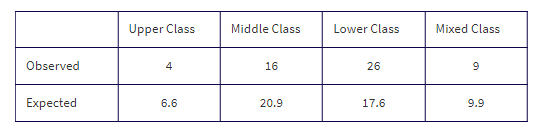
First, state the hypotheses.
H0:Liquor stores are distributed over the four city regions in the same proportions as the areas of those regions, that is, in the percentages 12, 38, 32, and 18, respectively.
Ha:Liquor stores are not distributed over the four city regions in the same proportions as the areas of those regions (at least one proportion is not as specified in the null hypothesis).
Second, name the procedure and check the conditions:
Procedure: A chi-square test for Goodness-of-fit.
Checks:
Randomization: We are given that the sample is random.
We note that the expected values (6.6, 20.9, 17.6, 9.9) are all > 5.
We assume the sample size, 55, is less than 10% of the number of all liquor stores in the large city.
Third, calculate the Χ² statistic:
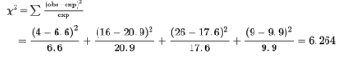
The P-value is P = P(χ2 > 6.264) = 0.099. [If n is the number of classes, df = n − 1 = 3, and χ2cdf(6.264, 1000, 3) = 0.099.] We also note that putting the observed and expected numbers in Lists, calculator software (such as χ2GOF-Test on the TI-84 or on the Casio Prizm) quickly gives χ2 = 6.262 and P = 0.099.
Fourth, give a conclusion in context with linkage to the P-value:
With this large a P-value, 0.099 > 0.05, there is not sufficient evidence to reject H0. That is, there is not convincing evidence that liquor stores in this city are distributed over the four city regions (upper, middle, lower, and mixed class) in different proportions to the areas of those regions.
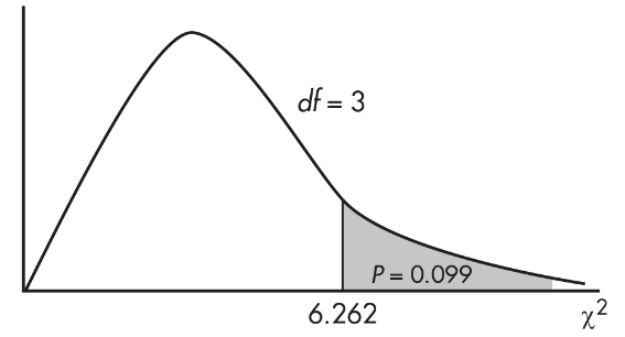
Chi-Square Test for Independence
Test of Independence - There is a class of real-world problems in which we want to determine if there is a significant association between two categorical variables.
We classify our single sample observations in two ways and then ask whether the two ways are independent of each other.
For example, we might consider several age groups and within each group ask how many employees show various levels of job satisfaction. The null hypothesis is that age and job satisfaction are independent, that is, that the proportion of employees expressing a given level of job satisfaction is the same no matter which age group is considered.
When testing for independence,
![]()
where df is the number of degrees of freedom, r is the number of rows, and c is the number of columns.
A point worth noting is that even if there is sufficient evidence to reject the null hypothesis of independence, we cannot necessarily claim any direct causal relationship.
In other words, although we can make a statement about some link or relationship between two variables, we are not justified in claiming that one causes the other.
➥ Example 8.2
A growing number of states have legalized marijuana for medical or recreational purposes. In a nationwide telephone poll of 1000 randomly selected adults representing Democrats, Republicans, and Independents, respondents were asked two questions: their party affiliation and if they supported the legalization of marijuana. The answers, cross-classified by party affiliation, are given in the following two-way table (also called a contingency table).

Test the null hypothesis that support for legalizing marijuana is independent of party affiliation. Use a 5% significance level.
Solution:
Hypothesis H0:Party affiliation and support for legalizing marijuana are independent.
Ha:Party affiliation and support for legalizing marijuana are not independent.
Mechanics: Putting the observed data into a "Matrix," calculator software (such as χ2-Test on the TI-84, Casio Prizm, or HP Prime) gives χ2 = 94.5 and P = 0.000, and stores the expected values in a second matrix:
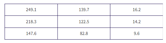
Check conditions: We are given a random sample, n = 1000 is less than 10% of all adults, and we note that all expected cells are > 5.
Conclusion with linkage to the P-value: With this small of a P-value, 0.000 < 0.05, there is sufficient evidence to reject H0; that is, among all adults there is sufficient evidence of a relationship between party affiliation and support for legalizing marijuana.
Chi-Square Test for Homogeneity
Chi-square procedures can also be used with a single variable to compare samples from two or more populations.
Conditions to check include that the samples be simple random samples, that they be taken independently of each other, that the original populations be large compared to the sample sizes, and that the expected values for all cells be at least 5. The contingency table used has a row for each sample. The resulting procedure is called a chi-square test for homogeneity.
➥ Example 8.3
In a large city, a group of AP Statistics students work together on a project to determine which group of school employees has the greatest proportion who are satisfied with their jobs. In independent simple random samples of 100 teachers, 60 administrators, 45 custodians, and 55 secretaries, the numbers satisfied with their jobs were found to be 82, 38, 34, and 36, respectively. Is there evidence that the proportion of employees satisfied with their jobs is different in different school system job categories?
Solution:
Hypotheses:
H0:The proportion of employees satisfied with their jobs is the same across the various school system job categories.
Ha:At least two of the job categories differ in the proportion of employees satisfied with their jobs.
Procedure: A chi-square test for homogeneity.
Checks:
We are given independent simple random samples (a stratified random sample).
The expected cells (calculated below) are all greater than 5.
We assume that the four samples are each less than 10% of their respective populations in the large city.
Mechanics: using Matrix and χ2-Test on a calculator, we find the expected cells, the test statistic χ2, and the P-value.
The observed counts are as follows:
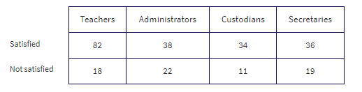
Putting the observed data into a Matrix, calculator software gives χ2 = 8.707 and P = 0.0335 and stores the expected values in a second matrix:
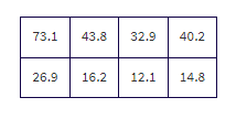
Conclusion in context with linkage to the P-value:
With this small of a P-value, 0.0335 < 0.05, there is sufficient evidence to reject H0; that is, there is convincing evidence that the true proportion of employees satisfied with their jobs is not the same across all the school system job categories.
Unit: 9 Inference for Quantitative Data: Slopes
Sampling Distribution for the Slope
When certain conditions are met, we can model the sampling distribution of the sample slope b with a normal distribution with mean μb and standard deviation σb. Working with the standard error sb as an estimate for σb leads to a t-distribution with df = n – 2.
If μy is the mean value of the response variable y for a given value of the explanatory variable x, then the population regression model is given by μy= α + βx.
The theoretical conditions for inference on the slope are
The true relationship between the response and explanatory variables is linear.
The standard deviation of y, σy, does not vary with x.
The responses (y-values) for each x are approximately normally distributed.
While the above are the theoretical conditions that should be met, we will be working with data from a single sample; therefore, we will be approximating the sampling distribution and need to give conditions based on the sample slope b, a standard deviation of the sample residuals s, and a standard deviation of the sample x-values sx. Using s and sx as estimates for σ and σx, respectively, leads us to estimating σb with sb and a resulting t-distribution with df = n – 2. That is, the statistic
has a t-distribution with df = n – 2.
Fortunately,
![]()
= standard error of the sample slopes is typically given to you in generic computer output.
Confidence Interval for the Slope of a Least Squares Regression Line
The slope b of the regression line and the standard error

of the slope are listed explicitly in the computer output. A confidence interval for β can be found using t-scores with df = n − 2.
If given raw data, a confidence interval can readily be found using the statistical software on a calculator.
Conditions for finding a confidence interval for the slope include:
The sample must be randomly selected.
The scatterplot should be approximately linear.
There should be no apparent pattern in the residuals plot.
The distribution of the residuals should be approximately normal.
The sample size n should be less than 10 percent of the population size N.
➥ Example 9.1
Information concerning SAT verbal scores and SAT math scores was collected from 15 randomly selected students. A linear regression performed on the data using a statistical software package produced the following printout:
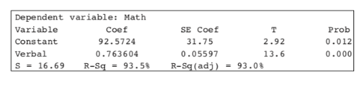
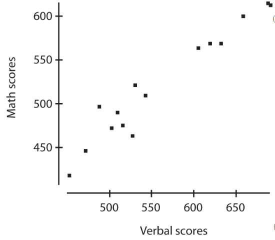
Assume that all conditions for regression are met. What is the regression equation?
What is a 95% confidence interval estimate for the slope of the regression line?
Does the confidence interval (0.64 to 0.89) provide convincing evidence that SAT math scores are linearly related to SAT verbal scores?
Solution:
The y-intercept and slope of the equation are found in the Coefcolumn of the above printout.
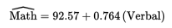
Parameter: Let β represent the slope of the true regression line for predicting SAT math scores from SAT verbal scores.
Procedure: One-sample t-interval for β
Conditions: Given that all conditions are met
Mechanics: The standard deviation of the residuals is S = 16.69 and the standard error of the slope is
![]()
With 15 data points, df = 15 − 2 = 13, and the critical t-values are ±invT(0.975, 13) = ±2.160. The 95% confidence interval of the true slope is:
![]()
Conclusion in context: We are 95% confident that the interval from 0.64 to 0.89 captures the slope of the true regression line relating the SAT math score, y, and SAT verbal score, x. (Or we are 95% confident that for every 1-point increase in verbal SAT score, the average increase in math SAT score is between 0.64 and 0.89.) provide convincing evidence that SAT math scores are linearly related to SAT verbal scores?
Note that β = 0 would indicate a line with slope 0 is the model for predicting SAT math scores from SAT verbal scores; that is, the model would predict the same SAT math score no matter what the SAT verbal score, and there would not be convincing evidence of a linear relationship.
In this example, because the confidence interval (0.64 to 0.89) does not contain 0 as a plausible value of the slope of the population regression line, there is convincing evidence that SAT math and verbal scores are linearly related.
Hypothesis Test for Slope of Least Squares Regression Line
In addition to finding a confidence interval for the true slope, we can also perform a hypothesis test for the value of the slope. Often we use the null hypothesis H0: β = 0, that is, that there is no linear relationship between the two variables.
Assumptions for inference for the slope of the least squares line include the following:
The sample must be randomly selected.
The scatterplot should be approximately linear.
There should be no apparent pattern in the residuals plot.
The distribution of the residuals should be approximately normal.
The sample size n should be less than 10 percent of the population size N.
Note that a low P-value tells us that if the two variables did not have some linear relationship, it would be highly unlikely to find such a random sample. However, strong evidence that there is some linear association does not mean the association is strong.
➥ Example 9.3
The following table gives serving speeds in mph (using a flat or “cannonball” serve) of ten randomly selected professional tennis players before and after using a newly developed tennis racket.
Is there evidence of a straight-line relationship with positive slope between serving speeds of professionals using their old and the new rackets?
Interpret in context the least squares line.
Solution:
Parameter: Let β represent the slope of the true regression line for predicting serving speed in mph after using a newly developed tennis racket from serving speed before using a newly developed tennis racket.
Hypotheses: H0: β = 0, Ha: β > 0.
Procedure: t-test for the slope of a regression line.
Checks: We are told that the data come from a random sample of professional players, the scatterplot appears to be approximately linear, there is no apparent pattern in the residuals plot, the histogram of residuals appears to be approximately normal, and the sample of size 10 is less than 10% of all professional players.
Mechanics: Using the statistics software on a calculator (for example, LinRegTTest on the TI-84 or LinearReg tTest on the Casio Prizm) gives:
![]()
Conclusion in context with linkage to the P-value:
With such a small P-value, 0.00019 < 0.05, there is very strong evidence to reject H0; that is, there is convincing evidence of a straight-line relationship with positive slope between serving speeds of professionals using their old and the new rackets.
With a slope of approximately 1 and a y-intercept of 8.76, the regression line indicates that use of the new racket increases serving speed on the average by 8.76 mph regardless of the old racket speed. That is, players with lower and higher old racket speeds experience on the average the same numerical (rather than percentage) increase when using the new racket.