
Unit 6: Inference for Categorical Data: Proportions
The Meaning of a Confidence Interval
The percentage is the percentage of samples that would pinpoint the unknown p or µ within plus or minus respective margins of error.
For a given sample proportion or mean, p or µ either is or isn’t within the specified interval, and so the probability is either 1 or 0.
Two aspects to this concept:
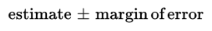
First, there is the confidence interval, usually expressed in the form:
Second, there is the success rate for the method, called the confidence level, that is, the proportion of times repeated applications of this method would capture the true population parameter.
The standard error is a measure of how far the sample statistic typically varies from the population parameter.
The margin of error is a multiple of the standard error, with that multiple determined by how confident we wish to be of our procedure.
All of the above assume that certain conditions are met. For inference on population proportions, means, and slopes, we must check for independence in data collection methods and for selection of the appropriate sampling distribution.
Conditions for Inference
The following are the two standard assumptions for our inference procedures and the "ideal" way they are met:
Independence assumption:
Individuals in a sample or an experiment an must be independent of each other, and this is obtained through random sampling or random selection.
Independence across samples is obtained by selecting two (or more) separate random samples.
Always examine how the data were collected to check if the assumption of independence is reasonable.
Sample size can also affect independence. Because sampling is usually done without replacement, if the sample is too large, lack of independence becomes a concern.
So, we typically require that the sample size n be no larger than 10% of the population (the 10% Rule).
Normality assumption:
Inference for proportions is based on a normal model for the sampling distribution of p̂, but actually we have a binomial distribution.
Fortunately, the binomial is approximately normal if both np and nq ≥ 10.
Inference for means is based on a normal model for the sampling distribution of x̄; this is true if the population is normal and is approximately true (thanks to the CLT) if the sample size is large enough (typically we accept n ≥ 30).
With regard to means, this is referred to as the Normal/Large Sample condition.
➥ Example 6.1
If we pick a simple random sample of size 80 from a large population, which of the following values of the population proportion p would allow use of the normal model for the sampling distribution of p̂?
0.10
0.15
0.90
0.95
0.99
Solution: (B)
The relevant condition is that both np and nq ≥ 10.
In (A), np = (80)(0.10) = 8; in (C), nq = (80)(0.10) = 8; in (D), nq = (80)(0.05) = 4; and in (E), nq = (80)(0.01) = 0.8. However, in (B), np = (80)(0.15) = 12 and nq = (0.85)(80) = 68 are both ≥ 10.
Confidence Interval for a Proportion
Estimating a population proportion p by considering a single sample proportion p̂.
This sample proportion is just one of a whole universe of sample proportions, and from Unit 5 we remember the following:
The set of all sample proportions is approximately normally distributed.
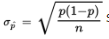
The mean μp̂ of the set of sample proportions equals p, the population proportion.
The standard deviation σp̂ of the set of sample proportions is approximately equal to

In finding confidence interval estimates of the population proportion p, how do we find
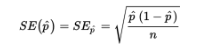
since p is unknown? The reasonable procedure is to use the sample proportion p̂:
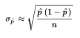
When the standard deviation is estimated in this way (using the sample), we use the term standard error:
 ➥ Example 6.2
If 42% of a simple random sample of 550 young adults say that whoever asks for the date should pay for the first date, determine a 99% confidence interval estimate for the true proportion of all young adults who would say that whoever asks for the date should pay for the first date.
Does this confidence interval give convincing evidence in support of the claim that fewer than 50% of young adults would say that whoever asks for the date should pay for the first date?
Solution:
The parameter is p, which represents the proportion of the population of young adults who would say that whoever asks for the date should pay for the first date. We check that
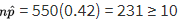

We are given that the sample is an SRS, and 550 is clearly less than 10% of all young adults. Since p̂ = 0.42, the standard error of the set of sample proportions is
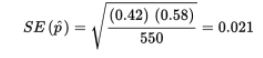
99% of the sample proportions should be within 2.576 standard deviations of the population proportion. Equivalently, we are 99% certain that the population proportion is within 2.576 standard deviations of any sample proportion.
Thus, the 99% confidence interval estimate for the population proportion is 0.42 ± 2.576(0.021) = 0.42 ± 0.054. We say that the margin of error is ±0.054. We are 99% confident that the true proportion of young adults who would say that whoever asks for the date should pay for the first date is between 0.366 and 0.474.
Yes, because all the values in the confidence interval (0.366 to 0.474) are less than 0.50, this confidence interval gives convincing evidence in support of the claim that fewer than 50% of young adults would say that whoever asks for the date should pay for the first date.
Logic of Significance Testing
Closely related to the problem of estimating a population proportion or mean is the problem of testing a hypothesis about a population proportion or mean.
The general testing procedure is to choose a specific hypothesis to be tested, called the null hypothesis, pick an appropriate random sample, and then use measurements from the sample to determine the likelihood of the null hypothesis.
If the sample statistic is far enough away from the claimed population parameter, we say that there is sufficient evidence to reject the null hypothesis. We attempt to show that the null hypothesis is unacceptable by showing that it is improbable.
The null hypothesis H0 is stated in the form of an equality statement about the population proportion (for example, H0: p = 0.37).
There is an alternative hypothesis, stated in the form of a strict inequality (for example, Ha: p < 0.37 or Ha: p > 0.37 or Ha: p ≠ 0.37).
The strength of the sample statistic p̂ can be gauged through its associated P-value, which is the probability of obtaining a sample statistic as extreme (or more extreme) as the one obtained if the null hypothesis is assumed to be true. The smaller the P-value, the more significant the difference between the null hypothesis and the sample results.
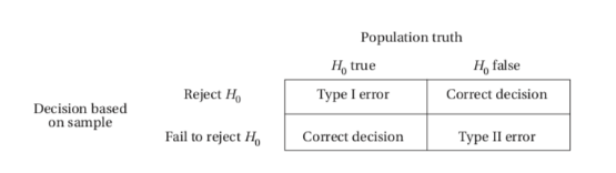
There are two types of possible errors:
the error of mistakenly rejecting a true null hypothesis.
the error of mistakenly failing to reject a false null hypothesis.
The α-risk, also called the significance level of the test, is the probability of committing a Type I error and mistakenly rejecting a true null hypothesis.
Type II error - a mistaken failure to reject a false null hypothesis, has associated probability β.
There is a different value of β for each possible correct value for the population parameter p. For each β, 1 − β is called the "power" of the test against the associated correct value.
Power of a hypothesis test - is the probability that a Type II error is not committed.
That is, given a true alternative, the power is the probability of rejecting the false null hypothesis. Increasing the sample size and increasing the significance level are both ways of increasing the power. Also note that a true null that is further away from the hypothesized null is more likely to be detected, thus offering a more powerful test.
A simple illustration of the difference between a Type I and a Type II error is as follows.
Suppose the null hypothesis is that all systems are operating satisfactorily with regard to a NASA launch. A Type I error would be to delay the launch mistakenly thinking that something was malfunctioning when everything was actually OK. A Type II error would be to fail to delay the launch mistakenly thinking everything was OK when something was actually malfunctioning. The power is the probability of recognizing a particular malfunction. (Note the complementary aspect of power, a “good” thing, with Type II error, a “bad” thing.)
It should be emphasized that with regard to calculations, questions like “What is the power of this test?” and “What is the probability of a Type II error in this test?” cannot be answered without reference to a specific alternative hypothesis.
Significance Test for a Proportion
It is important to understand that because the P-value is a conditional probability, calculated based on the assumption that the null hypothesis, H0: p = p0, is true, we use the claimed proportion p0 both in checking the np0 ≥ 10 and n(1 − p0) ≥ 10 conditions and in calculating the standard deviation 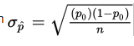
➥ Example 6.3
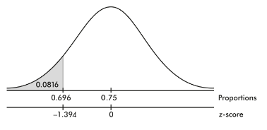
A union spokesperson claims that 75% of union members will support a strike if their basic demands are not met. A company negotiator believes the true percentage is lower and runs a hypothesis test. What is the conclusion if 87 out of a simple random sample of 125 union members say they will strike?
For each of the two possible answers above, what error might have been committed, Type I or Type II, and what would be a possible consequence?
Solution:
Parameter: Let p represent the proportion of all union members who will support a strike if their basic demands are not met.
Hypotheses: H0: p = 0.75 and Ha: p < 0.75.
Procedure: One-sample z-test for a population proportion.
Checks: np0 = (125)(0.75) = 93.75 and n(1 − p0) = (125)(0.25) = 31.25 are both ≥ 10, it is given that we have an SRS, and we must assume that 125 is less than 10% of the total union membership.
Mechanics: Calculator software (such as 1-PropZTest on the TI-84 or Z-1-PROP on the Casio Prizm) gives z = −1.394 and P = 0.0816.
Conclusion in context with linkage to the P-value: There are two possible answers:
a. With this large of a P-value, 0.0816 > 0.05, there is not sufficient evidence to reject H0; that is, there is not sufficient evidence at the 5% significance level that the true percentage of union members who support a strike is less than 75%.
b. With this small of a P-value, 0.0816 < 0.10, there is sufficient evidence to reject H0; that is, there is sufficient evidence at the 10% significance level that the true percentage of union members who support a strike is less than 75%.
If the P-value is considered large, 0.0816 > 0.05, so that there is not sufficient evidence to reject the null hypothesis, there is the possibility that a false null hypothesis would mistakenly not be rejected and thus a Type II error would be committed. In this case, the union might call a strike thinking they have greater support than they actually do. If the P-value is considered small, 0.0816 < 0.10, so that there is sufficient evidence to reject the null hypothesis, there is the possibility that a true null hypothesis would mistakenly be rejected, and thus a Type I error would be committed. In this case, the union might not call for a strike thinking they don’t have sufficient support when they actually do have support.
Confidence Interval for the Difference of Two Proportions
From Unit 5, we have the following information about the sampling distribution of 
The set of all differences of sample proportions is approximately normally distributed.
The mean of the set of differences of sample proportions equals p1 − p2, the difference of the population proportions.
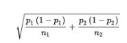
The standard deviation
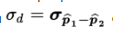
of the set of differences of sample proportions is approximately equal to:
Remember that we are using the normal approximation to the binomial, so
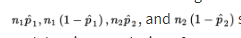
should all be at least 10. In making calculations and drawing conclusions from specific samples, it is important both that the samples be simple random samples and that they be taken independentlyof each other. Finally, the original populations should be large compared to the sample sizes, that is, check that
➥ Example 6.4
Suppose that 84% of a simple random sample of 125 nurses working 7:00 a.m. to 3:00 p.m. shifts in city hospitals express positive job satisfaction, while only 72% of an SRS of 150 nurses on 11:00 p.m. to 7:00 a.m. shifts express similar fulfillment. Establish a 90% confidence interval estimate for the difference.
Based on the interval, is there convincing evidence that the nurses on the 7 AM to 3 PM shift express a higher job satisfaction than nurses on the 11 PM to 7 AM shift?
Solution:
Parameters: Let p1 represent the proportion of the population of nurses working 7:00 a.m. to 3:00 p.m. shifts in city hospitals who have positive job satisfaction. Let p2 represent the proportion of the population of nurses working 11:00 p.m. to 7:00 a.m. shifts in city hospitals who have positive job satisfaction.
Procedure: Two-sample z-interval for a difference between population proportions, p1 − p2.
Checks:


we are given independent SRSs; and the sample sizes are assumed to be less than 10% of the populations of city hospital nurses on the two shifts, respectively.
Mechanics: 2-PropZInt on the TI-84 or 2-Prop ZInterval on the Casio Prizm give (0.0391, 0.2009).
The observed difference is 0.84 − 0.72 = 0.12, and the critical z-scores are ±1.645. The confidence interval estimate is 0.12 ± 1.645(0.0492) = 0.12 ± 0.081.]
Conclusion in context: We are 90% confident that the true proportion of satisfied nurses on 7:00 a.m. to 3:00 p.m. shifts is between 0.039 and 0.201 higher than the true proportion for nurses on 11:00 p.m. to 7:00 a.m. shifts.
Yes, because the entire interval from 0.039 to 0.201 is positive, there is convincing evidence that the nurses on the 7 AM to 3 PM shift express a higher job satisfaction than nurses on the 11 PM to 7 AM shift.
Significance Test for the Difference of Two Proportions
The null hypothesis for a difference between two proportions is

and so the normality condition becomes that
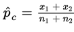
 should all be at least 10, where p̂ is the combined (or pooled) proportion,
  The other important conditions to be checked are both that the samples be random samples, ideally simple random samples, and that they be taken independently of each other. The original populations should also be large compared to the sample sizes, that is, check that
Two points need to be stressed:
First, sample proportions from the same population can vary from each other.
Second, what we are really comparing are confidence interval estimates, not just single points.
For many problems, the null hypothesis states that the population proportions are equal or, equivalently, that their difference is 0:
The alternative hypothesis is then:
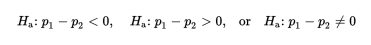
where the first two possibilities lead to one-sided tests and the third possibility leads to a two-sided test.
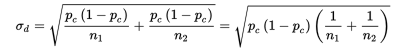
Since the null hypothesis is that p1 = p2, we call this common value pc and use this pooled value in calculating σd:
In practice, if
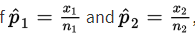
we use
as an estimate of pc in calculating σd.
➥ Example 6.5
In a random sample of 1500 First Nations children in Canada, 162 were in child welfare care, while in an independent random sample of 1600 non-Aboriginal children, 23 were in child welfare care. Many people believe that the large proportion of indigenous children in government care is a humanitarian crisis. Do the above data give significant evidence that a greater proportion of First Nations children in Canada are in child welfare care than the proportion of non-Aboriginal children in child welfare care?
Does a 95% confidence interval for the difference in proportions give a result consistent with the above conclusion?
Solution:
Parameters: Let p1 represent the proportion of the population of First Nations children in Canada who are in child welfare care. Let p2 represent the proportion of the population of non-Aboriginal children in Canada who are in child welfare care.
Hypotheses: H0: p1 − p2 = 0 or H0: p1 = p2 and Ha: p1 – p2 > 0 or Ha: p1 > p2.
Procedure: Two-sample z-test for a difference of two population proportions.
Checks: 
are all at least 10; the samples are random and independent by design; and it is reasonable to assume the sample sizes are less than 10% of the populations.
Mechanics: Calculator software (such as 2-PropZTest) gives z = 11.0 and P = 0.000.
Conclusion in context with linkage to the P-value: With this small of a P-value, 0.000 < 0.05, there is sufficient evidence to reject H0; that is, there is convincing evidence that that the true proportion of all First Nations children in Canada in child welfare care is greater than the true proportion of all non-Aboriginal children in Canada in child welfare care.
Calculator software (such as 2-PropZInt) gives that we are 95% confident that the true difference in proportions (true proportion of all First Nations children in Canada in child welfare care minus the true proportion of all non-Aboriginal children in Canada in child welfare care) is between 0.077 and 0.110. Since this interval is entirely positive, it is consistent with the conclusion from the hypothesis test.