Normal Distribution Calculations

• The normal distribution - provides a valuable model for how many sample statistics vary, under repeated random sampling from a population.

• Calculations involving normal distributions are often made through z**-scores**, which measure standard deviations from the mean.

• On the TI-84, normalcdf(lowerbound, upperbound) gives the area (probability) between two z-scores, while invNorm(area) gives the z-score with the given area (probability) to the left. The TI-84 also has the capability of working directly with raw scores instead of z-scores. In this case, the mean and standard deviation must be given:

Normalcdf(lowerbound, upperbound, mean, standard deviation)invNorm(area, mean, standard deviation)

➥ Example 5.1

The life expectancy of a particular brand of lightbulb is roughly normally distributed with a mean of 1500 hours and a standard deviation of 75 hours.

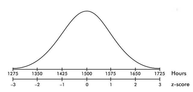
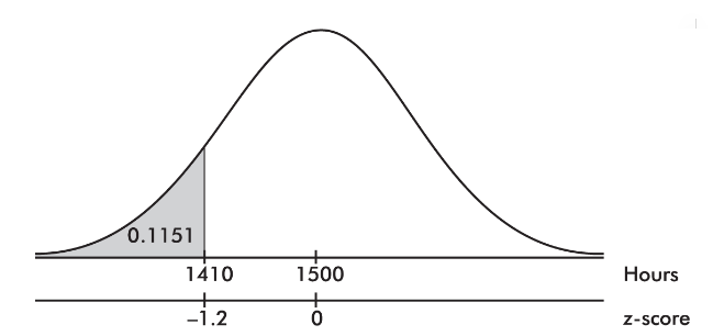
1. What is the probability that a lightbulb will last less than 1410 hours?

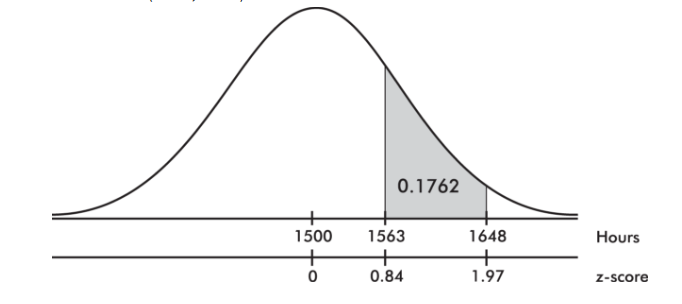
2. What is the probability that a lightbulb will last between 1563 and 1648 hours?

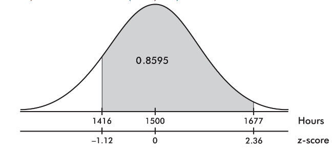
3. What is the probability that a lightbulb will last between 1416 and 1677 hours?

Solution:

1. The z-score of 1410 is

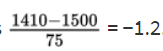
   On the TI-84, normalcdf(0, 1410, 1500, 75) = 0.1151 and normalcdf(−10, −1.2) = 0.1151.

   

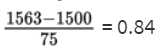
2. The z-score of 1563 is

   and the z-score of 1648 is

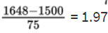
   Then we calculate the probability of between 1563 and 1648 hours by normalcdf(1563, 1648, 1500, 75) = 0.1762 or normalcdf(0.84, 1.97) = 0.1760.

   

   3. The z-score of 1416 is

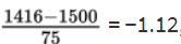
   and the z-score of 1677 is

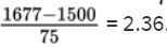
   Then we calculate the probability of between 1416 and 1677 hours by normalcdf(1416, 1677, 1500, 75) = 0.8595 or normalcdf(−1.12, 2.36) = 0.8595.

   

To receive full credit for probability calculations using the probability distributions, you need to show:

1. Name of the distribution ("normal" in the example above)

2. Parameters ("µ = 1500, σ = 75" in the example above)

3. Boundary ("1410" in (a) of the example above)

4. Values of interest ("<" in (a) of the example above)

5. Correct probability (0.1151 in (a) of the example above)

Central Limit Theorem

The following principle forms the basis of much of what we discuss in this unit and in those following. Statement 1 is called the central limit theorem of statistics (often simply abbreviated as CLT)

Start with a population with a given mean µ, a standard deviation σ, and any shape distribution whatsoever. Pick n sufficiently large (at least 30), and take all samples of size n. Compute the mean of each of these samples:

1. the set of all sample means is approximately normally distributed (often stated: the distribution of sample means is approximately normal).

2. the mean of the set of sample means equals µ, the mean of the population.

3. the standard deviation of the set of sample means is approximately equal to, that is, to the standard deviation of the whole population divided by the square root of the sample size.

Alternatively, we say that for sufficiently large n, the sampling distribution of x̄ is approximately normal with mean µ and standard deviation.

There are six key ideas to keep in mind:

• Averages vary less than individual values.

• Averages based on larger samples vary less than averages based on smaller samples.

• The central limit theorem (CLT) states that when the sample size is sufficiently large, the sampling distribution of the mean will be approximately normal.

• The larger the sample size n, the closer the sample distribution is to the population distribution.

• The larger the sample size n, the closer the sampling distribution of x̄ is to a normal distribution.

• If the original population has a normal distribution, then the sampling distribution of x̄ has a normal distribution, no matter what the sample size n.

➥ Example 5.2

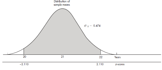
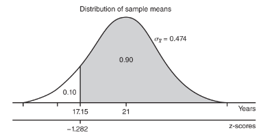
1. The naked mole rat, a hairless East African rodent that lives underground, has a life expectancy of 21 years with a standard deviation of 3 years. In a random sample of 40 such rats, what is the probability that the mean life expectancy is between 20 and 22 years?

2. The mean life expectancy is at least how many years with a corresponding probability of 0.90?

Solution:

We have a random sample that is less than 10% of the naked mole rat population. With a sample size of n = 40 ≥ 30, the central limit theorem applies, and the sampling distribution of x̄ is approximately normal with mean

and standard deviation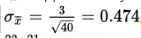

The z-scores of 20 and 22 are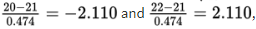

The probability of sample mean between 20 and 22 is normalcdf(–2.110,2.110)= 0.965. [Or normalcdf(20,22,21,0.474)= 0.965.]

2. The critical z-score is invNorm(0.10) = –1.282 with a corresponding raw score of 21 – 1.282(3) = 17.15 years.

Biased and Unbiased Estimators

• Bias means that the sampling distribution is not centered on the population parameter.

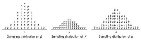
The sampling distributions of proportions, means, and slopes are unbiased*.* That is, for a given sample size, the set of all sample proportions is centered on the population proportion, the set of all sample means is centered on the population mean, and the set of all sample slopes is centered on the population slope.

Here are some illustrative simulations:

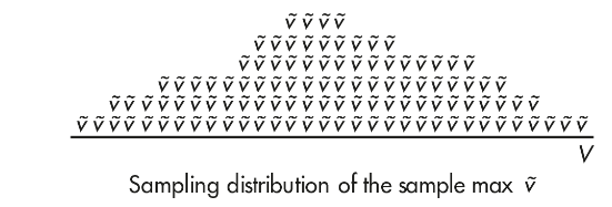
the sampling distribution for the maximum is clearly biased. That is, for a given sample size, the set of all sample maxima ṽ is not centered on the population maximum, V. For example, here is one simulation of sample maxima. Note that V falls far right of the center of the distribution of ṽ.

➥ Example 5.3

Five new estimators are being evaluated with regard to quality control in manufacturing professional baseballs of a given weight. Each estimator is tested every day for a month on samples of sizes n = 10, n = 20, and n = 40. The baseballs actually produced that month had a consistent mean weight of 146 grams. The distributions given by each estimator are as follows:

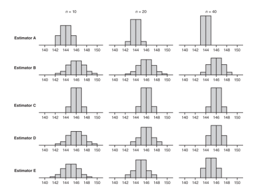
1. Which of the above appear to be unbiased estimators of the population parameter?

2. Which of the above exhibits the lowest variability for n = 40?

3. Which of the above is the best estimator if the selected estimator will eventually be used with a sample of size n = 100?

Solution:

1. Estimators B, C, and D are unbiased estimators because they appear to have means equal to the population mean of 146. A statistic used to estimate a population parameter is unbiased if the mean of the sampling distribution of the statistic is equal to the true value of the parameter being estimated.

2. For n = 40, estimator A exhibits the lowest variability, with a range of only 2 grams compared to the other ranges of 6 grams, 4 grams, 4 grams, and 4 grams, respectively.

3. Estimator D because we should choose an unbiased estimator with low variability. From part (a), we have Estimator B, C, and D as unbiased estimators. Now we look at the variability of these three statistics. As n increases, D shows tighter clustering around 146 than does B. Finally, while C looks better than D for n = 40, the estimator will be used with n = 100, and the D distribution is clearly converging as the sample size increases while the C distribution remains the same. Choose Estimator D.

Sampling Distribution for Sample Proportions

• The proportion essentially represents a qualitative calculation.

• The interest is simply in the presence or absence of some attribute.

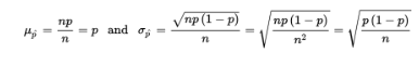
• Suppose the sample size is n and the actual population proportion is p. From our work on binomial distributions, we remember that the mean and standard deviation for the number of successes in a given sample are np and √np(1-p), respectively, and for large values of n the complete distribution begins to look “normal.”

• Here, however, we are interested in the proportion rather than in the number of successes. From Unit 1, remember that when we multiply or divide every element by a constant, we multiply or divide both the mean and the standard deviation by the same constant. In this case, to change number of successes to proportion of successes, we divide by n:

➥ Example 5.4

It is estimated that 80% of people with high math anxiety experience brain activity similar to that experienced under physical pain when anticipating doing a math problem. In a simple random sample of 110 people with high math anxiety, what is the probability that less than 75% experience the physical pain brain activity?

Solution:

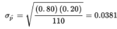
The sample is given to be random, both np = (110)(0.80) = 88 ≥ 10 and n(1 − p) = (110)(0.20) = 22 ≥ 10, and our sample is clearly less than 10% of all people with math anxiety. So, the sampling distribution of p̂ is approximately normal with mean 0.80 and standard deviation

With a z-score of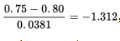

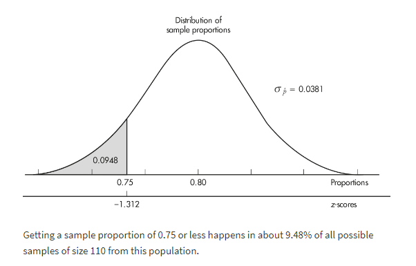
the probability that the sample proportion is less than 0.75 is normalcdf(–1000,–1.312) = 0.0948.

[Or normalcdf(–1000, 0.75, .80, .0381) = 0.0947.]

Sampling Distribution for Differences in Sample Proportions

• Dealing with one difference from the set of all possible differences obtained by subtracting sample proportions of one population from sample proportions of a second population.

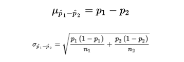
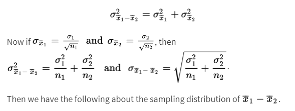
• To judge the significance of one particular difference, we must first determine how the differences vary among themselves. Remember that the mean of a set of differences is the difference of the means, and the variance of a set of differences is the sum of the variances of the individual sets.

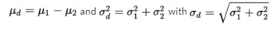
With our proportions we have 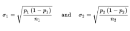   and can calculate:

➥ Example 5.5

In a study of how environment affects our eating habits, scientists revamped one of two nearby fast-food restaurants with table cloths, candlelight, and soft music. They then noted that at the revamped restaurant, customers ate more slowly and 25% left at least 100 calories of food on their plates. At the unrevamped restaurant, customers tended to quickly eat their food and only 19% left at least 100 calories of food on their plates. In a random sample of 110 customers at the revamped restaurant and an independent random sample of 120 customers at the unrevamped restaurant, what is the probability that the difference in the percentages of customers in the revamped setting and the unrevamped setting is more than 10% (where the difference is the revamped restaurant percent minus the unrevamped restaurant percent)?

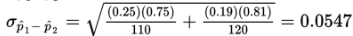
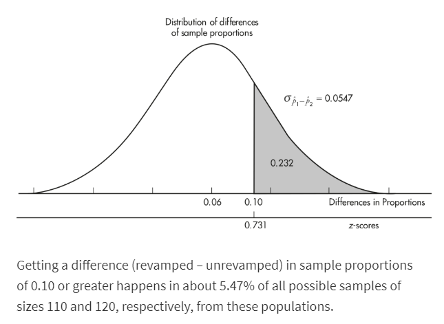
Solution: We have independent random samples, each less than 10% of all fast-food customers, and we note that n1p1 = 110(0.25) = 27.5, n1(1 − p1) = 110(0.75) = 82.5, n2p2 = 120(0.19) = 22.8, and n2(1 − p2) = 120(0.81) = 97.2 are all ≥10. Thus, the sampling distribution of p̂1- p̂2 is roughly normal with mean

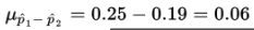
and standard deviation

The z-score of 0.10 is 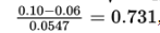, and normalcdf(0.731,1000)= 0.232. [Or normalcdf(0.10,1.0,0.06,0.0547)= 0.232.]

Sampling Distribution for Sample Means

• Suppose the variance of the population is σ2 and we are interested in samples of size n. Sample means are obtained by first summing together n elements and then dividing by n.

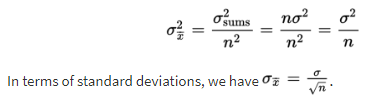
A set of sums has a variance equal to the sum of the variances associated with the original sets. In our case, 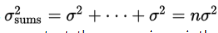When each element of a set is divided by some constant, the new variance is the old one divided by the square of the constant. Since the sample means are obtained by dividing the sums by n, the variance of the sample means is obtained by dividing the variance of the sums by n2. Thus, if σx̄ symbolizes the standard deviation of the sample means, we find that:

➥ Example 5.6

The number of emergency room visits after drinking energy drinks is skyrocketing. One particular energy drink has an average of 200 mg of caffeine with a standard deviation of 10 mg. A store sells boxes of six bottles each. What is the mean and standard deviation of the average milligrams of caffeine consumers should expect from the six bottles in each box?

Solution: We have samples of size 6, and 6 is assumed to be less than 10% of all such bottles. The mean of these sample means will equal the population mean of 200 mg. The standard deviation of these sample means will equal 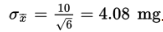 For all random samples of size n = 6 from this population, the sample mean milligrams of caffeine will have a mean of 200 mg and will typically vary by about 4.08 mg from the population mean of 200 mg.

Sampling Distribution for Differences in Sample Means

• To judge the significance of one particular difference, we must first determine how the differences vary among themselves.

• The necessary key is the fact that the variance of a set of differences is equal to the sum of the variances of the individual sets. Thus:

➥ Example 5.7

It is estimated that 40-year-old men contribute an average of 65 genetic mutations to their new children, whereas 20-year-old men contribute an average of only 25. Assuming standard deviations of 15 and 5 mutations, respectively, for the 40- and 20-year-olds, what is the probability that the mean number of mutations in a random sample of thirty-five 40-year-old new fathers is between 35 and 45 more than the mean number in a random sample of forty 20-year-old new fathers?

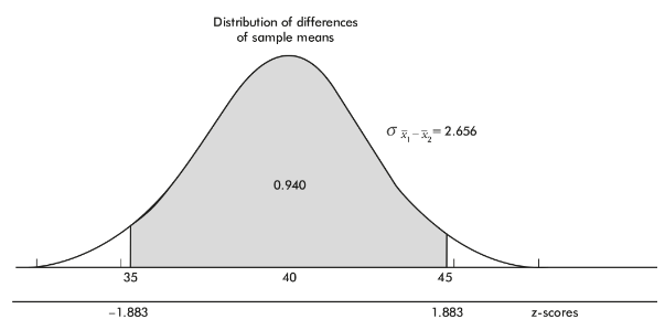
Solution: We have independent random samples, each less than 10% of their age groups, and both sample sizes are over 30, so the sampling distribution of x̄1-x̄2 is roughly normal with mean and standard deviation 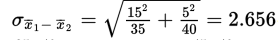The z-scores of 35 and 45 are , respectively, and normalcdf(-1.883,1.883)= 0.940. [Or normalcdf(35,45,40,2.656)= 0.940.]

Simulation of a Sampling Distribution

• The normal distribution can handle sampling distributions of the statistics we are most interested in, namely the sample proportion and sample mean.

• If other statistics arise, we can use simulation to obtain a rough idea of the corresponding sampling distributions.

For example, a study is made of the number of dreams high school students remember having every night. The median number is 3.41 with a variance of 1.46 and a minimum of 0. Now taking a large number of random samples of 15 students, we calculate the median, variance, and minimum for each sample and graph the resulting simulated sampling distributions.

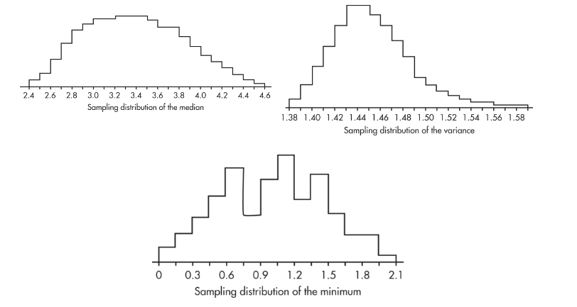
The simulated sampling distribution of these medians is roughly bell-shaped, the simulated sampling distribution of the variances is skewed right, and the simulated sampling distribution of the minimums is very roughly bell-shaped.