In this chapter, we will look at inference for categorical variables.

Chi-Square Tests

Example:

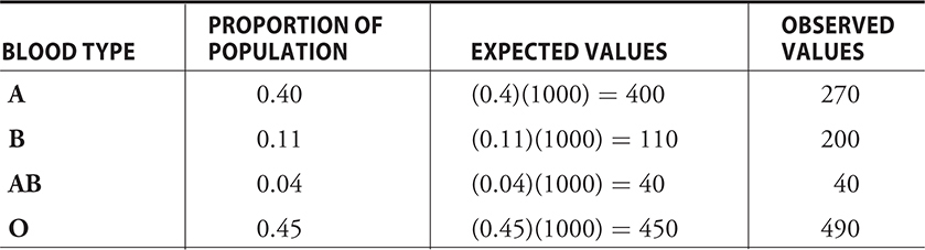
These are the approximate percentages for the different blood types among people with blue eyes: A: 40%; B: 11%; AB: 4%; O: 45%.

A random sample of 1000 people with brown eyes yielded the following blood type data:

A: 270; B: 200; AB: 40; O: 490.

Does this sample provide evidence that the distribution of blood types among brown-eyed people differs from that of blue-eyed people, or could the sample values simply be due to sampling variation?

• Chi Square goodness of fit test can be used to answer these questions.

• In the Chi-square goodness-of-fit test, there is one categorical variable (here : blood type) and one population(here : brown eyed people).

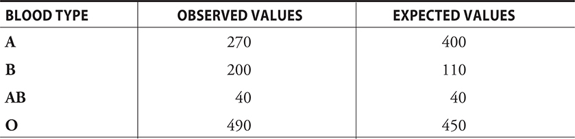
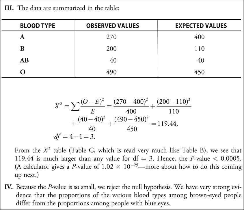
Comparing observed and expected values of the data, we get the following table:

The numbers vary for types A and B but not for types AB and O.

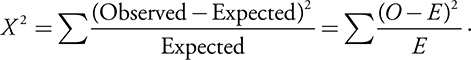
• The chi-square statistic ( X2 ) calculates the squared difference between the observed and expected values relative to the expected value for each category.

• The X2 statistic is computed as follows:

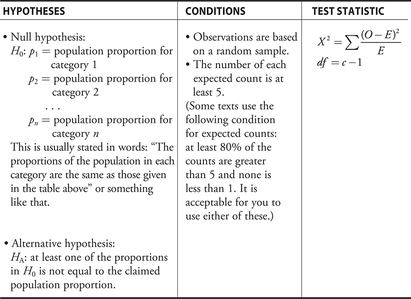
• The chi-square distribution is based on the number of degrees of freedom.

• degrees of freedom = (c − 1) where c is the number of categories.

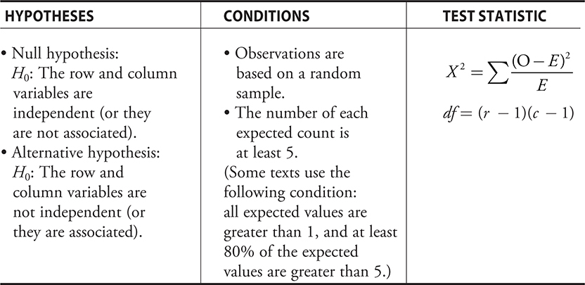
The essential parts of the test are summarized in the following table.

Now, assume

Pa = proportion of brown eyed people with type A blood.

Pb = proportion of brown eyed people with type B blood.

Pab = proportion of brown eyed people with type AB blood.

H0: Pa=0.4, Pb=0.11, Pab=0.45

Ha: Any of the above proportions is not as stated.

Using Chi-square Goodness-of-Fit test, expected values are as follows:

type A = 400

type B = 110

type AB = 40

type O = 450

Each is >5 and so the test is valid.

• In Chi-square test for homogeneity of proportions we may also encounter a situation in which there is one categorical variable measured across two or more populations

• Chi-square test for independence is one in which there are two categorical variables measured across a single population.

Inference for 2 Way Tables

• Two-Way Table or Contingency Table for categorical data is simply a rectangular array of cells.

• Each cell contains the frequencies for the joint values of the row and column variables.

• If the row variable has r values, then there will be r rows of data in the table.

• If the column variable has c values, then there will be c columns of data in the table.

• There are r × c cells in the table.

• The marginal totals are the sums of the observations for each row and each column.

• For a two-way table, the number of degrees of freedom is calculated as

====( number of rows – 1)( number of columns – 1) =====

( r − 1)( c − 1).

Chi-Square Test for Independence

The Chi-Squared test for independence is summarized as follows:

Chi-Square Test for Homogeneity of Proportions

• In this method, we use chi-square statistic to investigate whether or not the values of a single categorical variable are proportional among two or more populations.

Example:

Let’s consider a situation in which a sample of 36 students is selected and then categorized according to gender and political party preference. We then asked if gender and party preference are independent in the population.

Now suppose we selected a random sample of 20 males from the population of males in the school and another, independent, random sample of 16 females from the population of females in the school. Within each sample we classify the students as Democrat, Republican, or Independent. The results are presented in the following table:

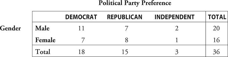
Here, we do not ask if gender and political party preference are independent. Instead, we ask if the proportions of Democrats, Republicans, and Independents are the same within the populations of Males and Females. This is the test for homogeneity of proportions.

Assume:

p1: proportion of Male Democrats

p2 : proportion of Female Democrats

p3: proportion of Male Republicans

p4: proportion of Female Republicans

p5: proportion of Independent Males

p6: proportion of Independent Females

Therefore:

H0 : p1=p2, p3=p4, p5=p6

HA : At least one of these proportions is not as specified.

Continue solving after this as followed in previous examples.

Click the link to go to the next chapter:

Chapter 12