The t-distribution

• When the population standard deviation σ is unknown, we use the sample standard deviation s as an estimate for σ.

• This Student’s t-distribution - was introduced in 1908 by W. S. Gosset, a British mathematician employed by the Guinness Breweries.

For a sample from a normally distributed population, we work with the variable

with a resulting t-distribution that is bell-shaped and symmetric but lower at the mean, higher at the tails, and so more spread out than the normal distribution.

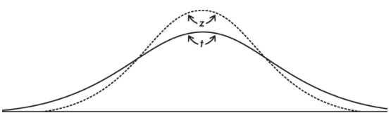
• The t-distribution is different for different values of n.

• In the tables, these distinct t-distributions are associated with the values for degrees of freedom (df).

For this discussion, the df value is equal to the sample size minus 1. The smaller the df value, the larger the dispersion in the distribution. The larger the df value, that is, the larger the sample size, the closer the distribution to the normal distribution.

• Thus, the t-distribution is the proper choice whenever the population standard deviation σ is unknown.

• In the real world, σ is almost always unknown, and so we should almost always use the t-distribution.

Confidence Interval for a Mean

This sample mean is just one of a whole universe of sample means, and we remember that if n is sufficiently large:

1. the set of all sample means is approximately normally distributed.

2. the mean of the set of sample means equals µ, the mean of the population.

3. the standard deviation of the set of sample means is approximately equal to , that is, equal to the standard deviation of the whole population divided by the square root of the sample size.

• Typically we do not know σ, the population standard deviation. In such cases, we must use s, the standard deviation of the sample, as an estimate of σ.

• In this case

  

is called the standard error

, and is used as an estimate for

➥ Example 7.1

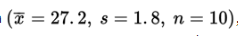
When a random sample of 10 cars of a new model was tested for gas mileage, the results showed a mean of 27.2 miles per gallon with a standard deviation of 1.8 miles per gallon.

1. What is a 95% confidence interval estimate for the mean gas mileage achieved by this model? (Assume that the population of mpg results for all the new model cars is approximately normally distributed.)

2. Based on this confidence interval, do you think that the true mean mileage is significantly different from 25 mpg?

3. Determine a 99% confidence interval.

4. What would the 95% confidence interval be if the sample mean of 27.2 and standard deviation of 1.8 had come from a sample of 20 cars?

5. With the original data

, with what confidence can we assert that the true mean gas mileage is 27.2 ± 1.04?

Solution:

1. Parameter: Let μ represent the mean gas mileage (in miles per gallon) in the population of cars of a new model.

Procedure: A one-sample t-interval for a population mean.

Checks: The sample is given to be random, 10 cars are assumed to be less than 10% of all cars of the new model, and the population is stated to be approximately normal. So,

follows a t-distribution.

Mechanics: Calculator software (such as TInterval on the TI-84 or 1-Sample tInterval on the Casio Prizm) gives (25.912, 28.488).

Conclusion in context: We are 95% confident that the true mean gas mileage of all cars of the new model is between 25.91 and 28.49 miles per gallon.

2. Yes, because 25 is not in the interval of plausible values from 25.9 to 28.5, there is convincing evidence that the true mean mileage is significantly different from 25 mpg.

3. Here, TInterval gives (25.35, 29.05). We are 99% confident that the true mean gas mileage of all cars of the new model is between 25.35 and 29.05 miles per gallon. Note that when we want a higher confidence (99% instead of 95%), we have to settle for a larger, less specific interval (±1.85) instead of (±1.29).

4. Here, TInterval gives (26.36, 28.04). We are 95% confident that the true mean gas mileage of all cars of the new model is between 26.36 and 28.04 miles per gallon. Note that when the sample size increased (from n = 10 to n = 20), the same sample mean and standard deviation resulted in a narrower, more specific interval (±0.84) instead of (±1.29).

5. Converting ±1.04 to t-scores yields

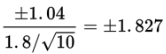
and tcdf(-1.827, 1.827, 9) = 0.899 = 89.9%. We are 89.9% confident that the true mean gas mileage of all cars of the new model is between 26.16 and 28.24 miles per gallon.

Significance Test for a Mean

• To conduct a significance test for a mean, we must check that we have a simple random sample, that the sample size is less than 10% of the population, and that either the sample size is large enough (n ≥ 30) for the CLT to apply or the population has an approximately normal distribution (either stated or if we are given the sample data, a plot should be unimodal and reasonably symmetric, showing no outliers and no skewness).

➥ Example 7.2

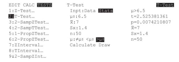
1. A manufacturer claims that a new brand of air-conditioning units uses only 6.5 kilowatts of electricity per day. A consumer agency believes the true figure is higher and runs a test on a random sample of size 50. If the sample mean is 7.0 kilowatts with a standard deviation of 1.4, should the manufacturer’s claim be rejected at a significance level of 5%? Of 1%?

2. Given the above conclusion, what type of error, Type-I or Type-II, might have been committed, and what would be a possible consequence?

Solution:

1. Parameter: Let μ represent the mean electricity usage (in kilowatts per day) of the population of a new brand of air-conditioning unit.

Hypotheses: H0: μ = 6.5 and Ha: μ > 6.5.

Procedure: A one-sample t-test for a population mean (population SD is unknown).

Checks: We are given a random sample, n = 50 ≥ 30 is large enough for the CLT to apply, and we can assume that 50 is less than 10% of all of the new AC units.

Mechanics: Calculator software (such as T-Test on the TI-84) gives t = 2.525 and P = 0.0074.

Conclusion in context with linkage to the P-value: With this small of a P-value, 0.0074 < 0.05, there is convincing evidence to reject H0; that is, there is sufficient evidence for the consumer agency to reject the manufacturer’s claim that the new unit uses a mean of only 6.5 kilowatts of electricity per day.

2. There was sufficient evidence to reject the null hypothesis. If the null hypothesis were true, we would be committing a Type-I error, that is, mistakenly rejecting a true null hypothesis. A possible consequence here is that the consumer agency would discourage customers from purchasing a new brand of air-conditioning unit that really was saving on electricity consumption as advertised.

Confidence Interval for the Difference of Two Means

We have the following information about the sampling distribution of

1. The set of all differences of sample means is approximately normally distributed.

2. The mean of the set of differences of sample means equals µ1 – µ2, the difference of population means.

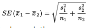
3. The standard deviation

of the set of differences of sample means is approximately equal to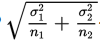

When the population standard deviations are unknown, use a t-distribution with

. There is the additional condition that either the original populations are roughly normal or the sample sizes are large enough (n1 ≥ 30 and n2 ≥ 30) for the CLT to apply.

➥ Example 7.3

1. A 30-month study is conducted to determine the difference in the numbers of accidents per month occurring in two departments in an assembly plant. Suppose the first department averages 12.3 accidents per month with a standard deviation of 3.5, while the second averages 7.6 accidents with a standard deviation of 3.4. Determine a 95% confidence interval estimate for the mean difference in the numbers of accidents per month. (Assume that the two populations are independent and approximately normally distributed.)

2. Based on this confidence interval, do you think that there is a significant mean difference (first department minus second department) in accidents per month between the two departments?

Solution:

1. Parameters: Let μ1 represent the mean number of accidents in the population of the number of accidents in all months for the first department. Let μ2 represent the mean number of accidents in the population of the number of accidents in all months for the second department.

Procedure: A two-sample t-interval for a difference between two population means (first department minus second department).

Checks: We are not given that the sample is random, so we must assume that the 30 months are representative. We are given that the two populations are independent and approximately normal, so a t-interval may be found (population SDs are unknown).

Mechanics: Calculator software (such as 2-SampTInt on the TI-84 or 2-Sample tInterval on the Casio Prizm) gives (2.9167, 6.4833).

Conclusion in context: We are 95% confident that the first department has a true mean of between 2.92 and 6.48 more accidents per month than the second department.

2. Yes, because the entire interval from 2.92 to 6.48 is positive, there is convincing evidence that the mean difference in accidents per month between the two departments is significant.

Significance Test for the Difference of Two Means

• A Significance test for the difference of two means requires us to check that we have two independent simple random samples and that either the original two populations are roughly normal or the sample sizes are each large enough (n1 ≥ 30 and n2 ≥ 30) for the CLT to apply.

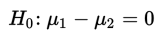
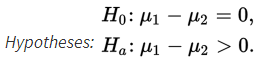
In this situation, the null hypothesis is usually that the means of the populations are the same or, equivalently, that their difference is 0:

The alternative hypothesis is then:

The first two possibilities lead to one-sided tests, and the third possibility leads to two-sided tests.

➥ Example 7.4

1. A sales representative believes that the computer his company sells has more average non-operational time per week than a similar model of computer sold by a competitor. Before taking this concern to his director, the sales representative gathers data and runs a significance test. He determines that in a simple random sample of 40 week-long periods at different firms using his company’s product, the average downtime was 125 minutes per week with a standard deviation of 37 minutes. However, 35 week-long periods involving the competitor’s computer yield an average downtime of only 115 minutes per week with a standard deviation of 43 minutes. What conclusion should the sales representative draw?

2. Given the above conclusion, what type of error, Type-I or Type-II, might have been committed, and what would be a possible consequence?

Solution:

1. Parameters: Let μ1 represent the mean of the population of non-operational times of the company's model computer. Let μ2 represent the mean of the population of non-operational times of the competitor's model computer.

Procedure: A two-sample t-test for the difference of two population means.

Checks: We are given independent SRSs, and the sample sizes are large enough (n1 = 40 ≥ 30 and n2 = 35 ≥ 30) for the CLT to apply. The population SDs are unknown, so a t-test is appropriate.

Mechanics: Calculator software gives t = 1.0718 and P = 0.1438.

Conclusion in context with linkage to the P-value: With this large of a P-value, 0.1438 > 0.05, there is not convincing evidence to reject H0; that is, the sales representative does not have convincing evidence that his company’s computers have greater mean non-operational time than that of the competitor’s computers.

2. There was not sufficient evidence to reject the null hypothesis. If the null hypothesis were false, we would be committing a Type-II error, that is, mistakenly failing to reject a false null hypothesis. A possible consequence here is that the company’s computers do have a greater mean non-operational time than those of the competitor’s, but because the test doesn’t show this, the company doesn’t make necessary fixes and future sales will suffer.

Paired Data

• When we have a quantitative variable measured twice for the same individual or for two very similar individuals, inference on the true mean difference involves one-sample analysis on the single variable consisting of the differences from the paired data.

➥ Example 7.5

An SAT preparation class of 30 randomly selected students produces the following total score summary:

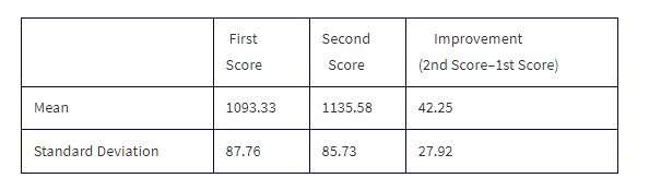
Find a 90% confidence interval of the mean improvement in test scores.

Solution: It would be wrong to calculate a confidence interval for a difference between two means using the means and standard deviations of the first and second scores. The independence condition between the two samples is violated! The proper procedure is a one-sample t-interval on the set of differences (improvement) between the scores for each of the 30 students.

Parameter: Let  μ represent the mean improvement (2nd score minus 1st score) in the SAT scores of the population of students who take this SAT preparation class.

Procedure: A one-sample t-interval for the mean of a population of differences in paired data.

Checks: We are given a random sample, n = 30 is less than 10% of all students, and n = 30 is large enough so that the CLT applies.

Mechanics: With an unknown population SD, it's necessary to find a t-interval.  Using  X̄ = 42.25 and s = 27.92, calculator software (such as TInterval) gives (33.59, 50.91).

Conclusion in context: We are 90% confident that the true mean improvement in test scores is between 33.59 and 50.91.

Simulations and P-Values

• We can use a simulation to determine what values of a test statistic are likely to occur by random chance alone, assuming the null hypothesis is true.

• Then looking at where our test statistic falls, we can estimate a P**-value**.

➥ Example 7.6

One measure of variability is the median absolute deviation (MAD). It is defined as the median deviation from the median, that is, as the median of the absolute values of the deviations from the median. A particular industrial product has the following quality control check. Random samples of size 6 are gathered periodically, and measurements are taken of the dimension under observation. If the MAD calculation is significantly greater than what is expected during proper operation of the machinery, a recalibration is necessary. In a simulation of 100 such samples of size 6 from when the machinery is working properly, the resulting MAD calculations are summarized in the following dotplot:

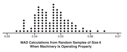
Suppose in a random sample of 6 products the measurements are {8.04, 8.06, 8.10, 8.14, 8.18, 8.19}. Is there sufficient evidence to necessitate a recalibration of the machinery?

Solution: The median is

. The absolute deviations from the median are {0.08, 0.06, 0.02, 0.02, 0.06, 0.07} with median

(the MAD calculation). In the simulation, there were 3 values out of 100 that were 0.06 or greater. This gives an estimated P-value of 0.03. With this small of a P-value, 0.03 < 0.05, there is sufficient evidence to necessitate a recalibration of the machinery.

More on Power, Type I Errors, and Type II Errors

• Type II error - is a mistaken failure to reject the false null hypothesis, while the power is the probability of rejecting that false null hypothesis.

➥ Example 7.7

A candidate claims to have the support of 70% of the people, but you believe that the true figure is lower. You plan to gather an SRS and will reject the 70% claim if your sample shows 65% or less support. What if, in reality, only 63% of the people support the candidate?

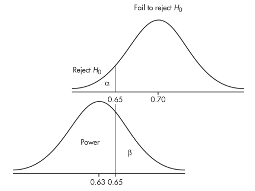
The upper graph shows the null hypothesis model with the claim that p0 = 0.70 and the plan to reject H0 if

The lower graph shows the true model with p = 0.63. When will we fail to recognize that the null hypothesis is incorrect? Answer: precisely when the sample proportion is greater than 0.65. This is a Type II error with probability β. When will we rightly conclude that the null hypothesis is incorrect? Answer: when the sample proportion is less than 0.65. This is the "power" of the test and has probability 1 − β.

Confidence Intervals Versus Hypothesis Tests

• A claim about a population parameter indicates a hypothesis test, while an estimate of a population parameter asks for a confidence interval.

➥ Example 7.8

Suppose it is reported that random samples of 3-point shots by basketball players Stephen Curry and Michael Jordan show a 43% rate for Curry and a 33% rate for Jordan.

(a) Are these numbers parameters or statistics?

(b) State appropriate hypotheses for testing whether the difference is statistically significant.

(c) Suppose the sample sizes were both 100. Find the z-statistic and the P-value, and give an appropriate conclusion at the 5% significance level.

(d) Calculate and interpret a 95% confidence interval for the difference in population proportions.

(e) Are the test decision and confidence interval consistent with each other?

(f) Repeat (c), (d), and (e) as if the sample size had been 200 for each.

Solutions:

(a) These two numbers are statistics because they describe  samples, not all 3-point shots ever taken by these two players.

(b) H0: pCurry = pJordan and Ha: pCurry ≠ pJordan.

(c) Calculator software gives z = 1.46 and P = 0.145. With this large of a P-value, 0.145 > 0.05, there is not sufficient evidence to reject H0; that is, there is not convincing evidence of a difference in the true 3-point percentage rates of Curry and Jordan.

(d) Calculator software gives (−0.034, 0.234). We are 95% confident that the true difference in 3-point percentage rates (Curry minus Jordan) is between −3.4% and 23.4%.

(e) Yes, they are consistent. We did not conclude that the two percentages differ, and the confidence interval (for the difference in population proportions) includes the value zero.

(f) With a sample size of 200, calculator software gives z = 2.06 and P = 0.039. With this small a P-value, 0.039 < 0.05, there is sufficient evidence to reject  H0; that is, there is convincing evidence of a difference in the true 3-point percentage rates of Curry and Jordan. With a sample size of 200, calculator software gives a confidence interval of (0.005, 0.195). We are 95% confident that the true difference in 3-point percentage rates (Curry minus Jordan) is between 0.5% and 19.5%. This interval does not include zero, so it is convincing evidence of a difference in the true 3-point percentage rates of Curry and Jordan. This is again consistent with the hypothesis test.