


Chapter 10: Inference for Regression
Simple Linear Regression
When doing inference for regression, we use ŷ =(a+bx) to estimate the true population regression line.
Similar to what we have done with other statistics used for inference, we use a and b as estimators of population parameters α and β , the intercept and slope of the population regression, respectively.
The conditions necessary for doing inference for regression are:
• For each given value of x , the values of the response variable y -values are independent and normally distributed. • For each given value of x , the standard deviation, σ , of y -values is the same. • The mean response of the y -values for the fixed values of x are linearly related by the equation µ y = α + βx

s is an estimator of σ,
(standard deviation of the residuals).
summary, inference for regression depends on estimating µy = α + βx with ŷ=a + bx .
Inference for regression depends on the following statistics:
a - the estimate of the y intercept, α , of µ
b - the estimate of the slope β , of µ y
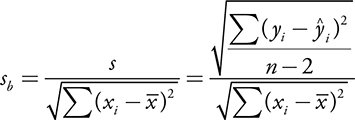
s - the standard error of the residuals
sb - the standard error of the slope of the regression line
Example:
The following data are pulse rates and heights for a group of 10 statistics students:
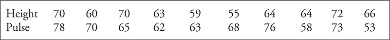
a. What is the least-squares regression line for predicting pulse rate from height? b. What is the correlation coefficient between height and pulse rate? Interpret the correlation coefficient in the context of the problem. c. What is the predicted pulse rate of a 67″ tall student? d. Interpret the slope of the regression line in the context of the problem.
Solution:
a) Pulse Rate = 47.17 +0.302(Height)
This equation can be found by entering the following on the TI-83/84:
L1=Height
L2=Pulse
STAT CALC LinReg(a+bx) L1,L2,Y1)
b) r = 0.21. There is a weak, positive, linear relationship between Height and pulse.
c) pulse rate = 47.17 + 0.302(67) = 67.4.
Again use the TI-83/84 and enter Y1(67)=67.42.
d) For a student one inch taller than another, the pulse rate is predicted to be an additional 0.302 beats per minute.
Inference for the Slope of a Regression Line
Inference for regression consists of either a significance test or a confidence interval for the slope of a regression line.
The null hypothesis in a significance test is
H0 : β = β0, but generally you will test H0 : β=0.
If the slope of the line is zero, then there is no linear relationship between the x and y variables.
The alternative hypothesis is often two sided.
HA : β ≠ 0.
We could do a one-sided test if we believed that the data were positively or negatively related.
Example:
The data in the following table give the top 15 states in terms of per-pupil expenditure in 1985 and the average teacher salary in the state for that year.
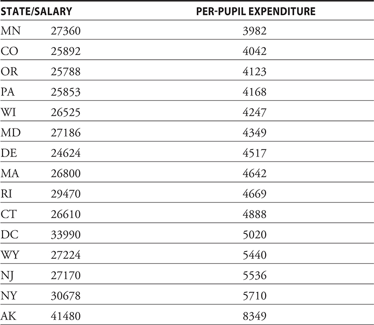
Test the hypothesis, at the 0.01 level of significance, that there is no straight-line relationship between per-pupil expenditure and teacher salary. Assume that the conditions necessary for inference for linear regression are present.
Solution:
Let β = true slope
Now, H0 : β=0 and HA : β ≠ 0.
The regression equation is:
Salary = 12027 +3.34PPE
(As s = 2281 and sb = 0.5536)
From this, the value of t and p-value can be found by :
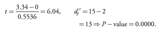
note: sb can be found by performing b/t.
As P value = 0 < α, we reject H0. The true slope of the line is thus not 0 and there is a linear relationship between amount of per-pupil expenditure and teacher salary.
A significance test that the slope of a regression line equals zero is closely related to a test that there is no correlation between the variables.
Confidence Interval for Slope of a Regression Line
We can construct a confidence interval for the true slope of a regression line.

Example:
Consider once again the earlier example on predicting teacher salary from per-pupil expenditure. Construct a 95% confidence interval for the slope of the population regression line.
Solution:
We found earlier that
Salary = 12027 +3.34PPE
Our confidence interval is of the form b ± t*sb .
We need to find t* and sb.
For C = 0.95 (95% confidence interval),
df = 15-2 = 13.
Now t=2.160.*
How to find: Use the invT function on your TI-83/84 and enter invT(0.975,13).
Now we can find sb:
sb= b/t =3.34/6.04=0.5530
Hence, b ± t*sb = 3.34±2.160(0.5530)=(2.15, 4.53).
We are 95% confident that the true slope of the regression line is between 2.15 and 4.53.
Inference for Regression Using Technology
Consider the following data that were gathered by counting the number of cricket chirps in 15 seconds and noting the temperature.

We can use technology to test the hypothesis that
slope of the regression line is 0 and to construct a confidence interval for the true slope of the regression line.
Computer regression output for the data:
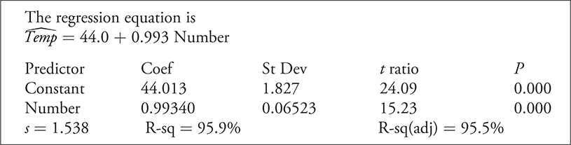
From this,
The regression equation:
Temp = 44.0+0.993(Number)
Predictor gives us the y-intercept and explanatory variable. These are Constant and Number respectively.
Coef gives values of the Constant and the slope of the regression line.
“Stdev” of “Number” is the standard error of the slope (sb).
s is the standard error of the residuals.
R-sq is the coefficient of determination (r^2)
Thus, all of the mechanics needed to do a t -test for the slope of a regression line are contained in this printout.
Click the link to go to the next chapter: