Introductory

• Bivariate data: two variable data

• Multivariate data: more than two variables

12.1 Linear Equations

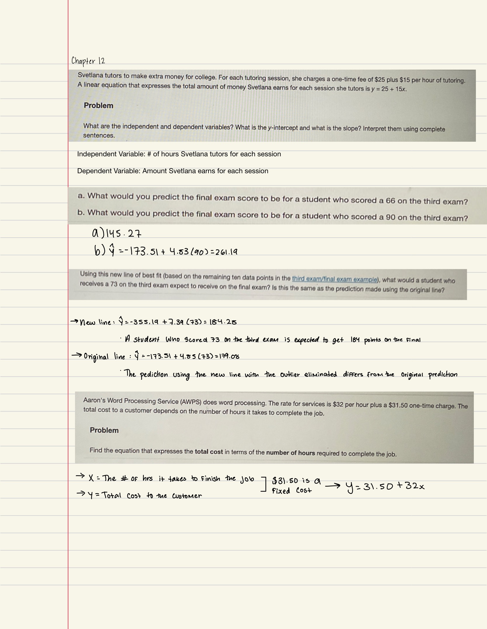
• y = a + bx: linear regression for two variables is based on a linear equation with one independent variable.

  • Independent variable: x

  • Dependent variable: y

  • Slope: b

  • y-intercept: a

• Graph form: a straight line or linear

  • B > 0: slopes to the right

  • b = 0: horizontal line

  • b < 0: slopes downward to the right

12.2 Scatter Plots

• Scatterplot: uses dots to represent values for two different numeric variables.

• Calculator steps for scatter plot

  • Enter your X data into list L1 and your Y data into list L2.

  • Press 2nd STATPLOT ENTER to use Plot 1. On the input screen for PLOT 1, highlight On and press ENTER. (Make sure the other plots are OFF.)

  • For TYPE: highlight the first icon, the scatter plot, and press ENTER.

  • For X List, enter L1 ENTER and for Ylist: L2 ENTER.

  • For Mark: it does not matter which symbol you highlight, but the square is the easiest to see. Press ENTER.

  • Make sure there are no other equations that could be plotted. Press Y = and clear any equations out.

  • Press the ZOOM key and then the number 9 (for menu item "ZoomStat"); the calculator will fit the window to the data. You can press WINDOW to see the scaling of the axes.

• Scatterplot Direction: High values of one variable occurring with high values of the other variable or low values of one variable occurring with low values of the other variable

• Strength: Looking at how close the points are to the line

• Linear regression: shows the relationship between a dependent and independent variable(s)

12.3 The Regression Equation

• Least-Squares Line: You have a set of data whose scatter plot appears to "fit" a straight line

• Least-squares regression line: Helps obtain a line of best fit

• y hat: estimates value of y

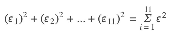
• y0 – ŷ0 = ε0: error or residual

• Absolute value of a residual: measures the vertical distance between the actual value of y and the estimated value of y

• ε: the Greek letter epsilon

• Slope equation: b = r (sy / sx)

  • sx = the standard deviation of the x values.

  • sy = the standard deviation of the y values

• Interpretation of the Slope: “The slope of the best-fit line tells us how the dependent variable (y) changes for every one unit increase in the independent (x) variable, on average.”

• Using the Linear Regression T Test

  • In the STAT list editor, enter the X data in list L1 and the Y data in list L2, paired so that the corresponding (x,y) values are next to each other in the lists.

  • On the STAT TESTS menu, scroll down with the cursor to select the LinRegTTest.

  • On the LinRegTTest input screen enter: Xlist: L1 ; Ylist: L2 ; Freq: 1

  • On the next line, at the prompt β or ρ, highlight "≠ 0" and press ENTER

  • Leave the line for "RegEq:" blank

  • Highlight Calculate and press ENTER.

• Correlation coefficient (r): is numerical and provides a measure of strength and direction of the linear association between the independent variable x and the dependent variable y.

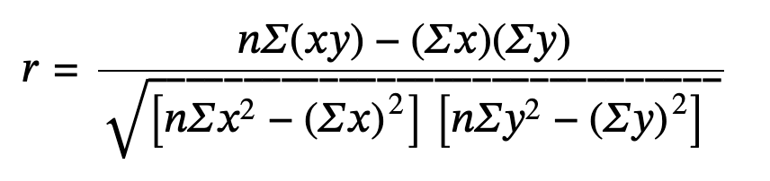
• The value of r is always between –1 and +1: –1 ≤ r ≤ 1.

• The size of the correlation r indicates the strength of the linear relationship between x and y. Values of r close to –1 or to +1 indicate a stronger linear relationship between x and y.

• If r = 0 there is likely no linear correlation. It is important to view the scatterplot, however, because data that exhibit a curved or horizontal pattern may have a correlation of 0.

• If r = 1, there is perfect positive correlation. If r = –1, there is perfect negative correlation. In both these cases, all of the original data points lie on a straight line.

• Positive correlation: A positive value of r means that when x increases, y tends to increase and when x decreases, y tends to decrease.

• Positive correlation: A negative value of r means that when x increases, y tends to decrease and when x decreases, y tends to increase

• Correlation does not imply causation

• 0 < r < 1: A scatter plot showing data with a positive correlation.

• –1 < r < 0: A scatter plot showing data with a negative correlation.

• r = 0: A scatter plot showing data with zero correlation.

• Coefficient of determination: a number between 0 and 1 that measures how well a statistical model predicts an outcome

• r^2 interpretation: when expressed as a percent, represents the percent of variation in the dependent (predicted) variable y that can be explained by variation in the independent (explanatory) variable x using the regression (best-fit) line.

• 1 - r^2 Interpretation: when expressed as a percentage, represents the percent of the variation in y that is NOT explained by variation in x using the regression line.

12.4 Testing the Significance of the Correlation Coefficient

• Significance of the correlation coefficient: to decide whether the linear relationship in the sample data is strong enough to use to model the relationship in the population.

• ρ: population correlation coefficient

• r: sample correlation coefficient

• Conclusion for Significant: There is sufficient evidence to conclude that there is a significant linear relationship between x and y because the correlation coefficient is significantly different from zero.

• Conclusion for Not Significant: There is insufficient evidence to conclude that there is a significant linear relationship between x and y because the correlation coefficient is not significantly different from zero.

• Null Hypothesis: H0→ ρ = 0

• Alternative Hypothesis: Ha→ ρ ≠ 0

• Interpreting Null Hypothesis: The population correlation coefficient IS NOT significantly different from zero. There IS NOT a significant linear relationship (correlation) between x and y in the population.

• Interpreting Alternate Hypothesis: The population correlation coefficient IS significantly DIFFERENT FROM zero. There IS A SIGNIFICANT LINEAR RELATIONSHIP (correlation) between x and y in the population.

• To calculate the p-value using LinRegTTEST

  • On the LinRegTTEST input screen, on the line prompt for β or ρ, highlight "≠ 0"

  • The output screen shows the p-value on the line that reads "p ="

• p-value is less than the significance level: We reject the null hypothesis. There is sufficient evidence to conclude that there is a significant linear relationship between x and y because the correlation coefficient is significantly different from zero

• p**-value is NOT less than the significance level**: DO NOT REJECT the null hypothesis. There is insufficient evidence to conclude that there is a significant linear relationship between x and y because the correlation coefficient is NOT significantly different from zero.

12.6 Outliers

• Outliers: are observed data points that are far from the least squares line.

• Influential points: observed data points that are far from the other observed data points in the horizontal direction. These points may have a big effect on the slope of the regression line.

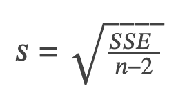
• Degrees of freedom: n - 2

Examples