

Chapter - 9 Inference for Quantitative Data: Slopes
Sampling Distribution for the Slope
When certain conditions are met, we can model the sampling distribution of the sample slope b with a normal distribution with mean μb and standard deviation σb. Working with the standard error sb as an estimate for σb leads to a t-distribution with df = n – 2.
If μy is the mean value of the response variable y for a given value of the explanatory variable x, then the population regression model is given by μy= α + βx.
The theoretical conditions for inference on the slope are
The true relationship between the response and explanatory variables is linear.
The standard deviation of y, σy, does not vary with x.
The responses (y-values) for each x are approximately normally distributed.
While the above are the theoretical conditions that should be met, we will be working with data from a single sample; therefore, we will be approximating the sampling distribution and need to give conditions based on the sample slope b, a standard deviation of the sample residuals s, and a standard deviation of the sample x-values sx. Using s and sx as estimates for σ and σx, respectively, leads us to estimating σb with sb and a resulting t-distribution with df = n – 2. That is, the statistic
has a t-distribution with df = n – 2.
Fortunately,
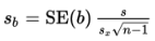
= standard error of the sample slopes is typically given to you in generic computer output.
Confidence Interval for the Slope of a Least Squares Regression Line
The slope b of the regression line and the standard error

of the slope are listed explicitly in the computer output. A confidence interval for β can be found using t-scores with df = n − 2.
If given raw data, a confidence interval can readily be found using the statistical software on a calculator.
Conditions for finding a confidence interval for the slope include:
The sample must be randomly selected.
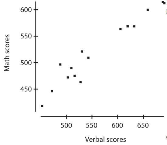
The scatterplot should be approximately linear.
There should be no apparent pattern in the residuals plot.
The distribution of the residuals should be approximately normal.
The sample size n should be less than 10 percent of the population size N.
➥ Example 9.1
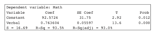
Information concerning SAT verbal scores and SAT math scores was collected from 15 randomly selected students. A linear regression performed on the data using a statistical software package produced the following printout:
Assume that all conditions for regression are met. What is the regression equation?
What is a 95% confidence interval estimate for the slope of the regression line?
Does the confidence interval (0.64 to 0.89) provide convincing evidence that SAT math scores are linearly related to SAT verbal scores?
Solution:
The y-intercept and slope of the equation are found in the Coefcolumn of the above printout.

Parameter: Let β represent the slope of the true regression line for predicting SAT math scores from SAT verbal scores.
Procedure: One-sample t-interval for β
Conditions: Given that all conditions are met
Mechanics: The standard deviation of the residuals is S = 16.69 and the standard error of the slope is
With 15 data points, df = 15 − 2 = 13, and the critical t-values are ±invT(0.975, 13) = ±2.160. The 95% confidence interval of the true slope is:

Conclusion in context: We are 95% confident that the interval from 0.64 to 0.89 captures the slope of the true regression line relating the SAT math score, y, and SAT verbal score, x. (Or we are 95% confident that for every 1-point increase in verbal SAT score, the average increase in math SAT score is between 0.64 and 0.89.) provide convincing evidence that SAT math scores are linearly related to SAT verbal scores?
Note that β = 0 would indicate a line with slope 0 is the model for predicting SAT math scores from SAT verbal scores; that is, the model would predict the same SAT math score no matter what the SAT verbal score, and there would not be convincing evidence of a linear relationship.
In this example, because the confidence interval (0.64 to 0.89) does not contain 0 as a plausible value of the slope of the population regression line, there is convincing evidence that SAT math and verbal scores are linearly related.
Hypothesis Test for Slope of Least Squares Regression Line
In addition to finding a confidence interval for the true slope, we can also perform a hypothesis test for the value of the slope. Often we use the null hypothesis H0: β = 0, that is, that there is no linear relationship between the two variables.
Assumptions for inference for the slope of the least squares line include the following:
The sample must be randomly selected.
The scatterplot should be approximately linear.
There should be no apparent pattern in the residuals plot.
The distribution of the residuals should be approximately normal.
The sample size n should be less than 10 percent of the population size N.
Note that a low P-value tells us that if the two variables did not have some linear relationship, it would be highly unlikely to find such a random sample. However, strong evidence that there is some linear association does not mean the association is strong.
➥ Example 9.3
The following table gives serving speeds in mph (using a flat or “cannonball” serve) of ten randomly selected professional tennis players before and after using a newly developed tennis racket.
Is there evidence of a straight-line relationship with positive slope between serving speeds of professionals using their old and the new rackets?
Interpret in context the least squares line.
Solution:
Parameter: Let β represent the slope of the true regression line for predicting serving speed in mph after using a newly developed tennis racket from serving speed before using a newly developed tennis racket.
Hypotheses: H0: β = 0, Ha: β > 0.
Procedure: t-test for the slope of a regression line.
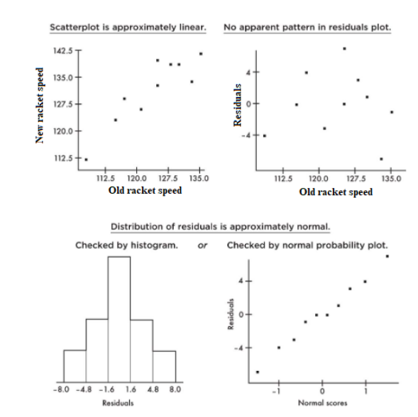
Checks: We are told that the data come from a random sample of professional players, the scatterplot appears to be approximately linear, there is no apparent pattern in the residuals plot, the histogram of residuals appears to be approximately normal, and the sample of size 10 is less than 10% of all professional players.
Mechanics: Using the statistics software on a calculator (for example, LinRegTTest on the TI-84 or LinearReg tTest on the Casio Prizm) gives:

Conclusion in context with linkage to the P-value:
With such a small P-value, 0.00019 < 0.05, there is very strong evidence to reject H0; that is, there is convincing evidence of a straight-line relationship with positive slope between serving speeds of professionals using their old and the new rackets.
With a slope of approximately 1 and a y-intercept of 8.76, the regression line indicates that use of the new racket increases serving speed on the average by 8.76 mph regardless of the old racket speed. That is, players with lower and higher old racket speeds experience on the average the same numerical (rather than percentage) increase when using the new racket.