
Unit - 8 Inference for Categorical Data: Chi-Square
Chi-Square Test for Goodness-of-Fit
A perfect fit cannot be expected, and so we must look at discrepancies and make judgments as to the Goodness-of-fit.
There is the null hypothesis of a good fit, that is, the hypothesis that a given theoretical distribution correctly describes the situation, problem, or activity under consideration.
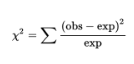
The sum of these weighted differences or discrepancies is called the chi-square statistic and is denoted as χ2 (χ is the lowercase Greek letter chi):
The smaller the resulting χ2-value, the better the fit.
The P**-value** is the probability of obtaining a χ2-value as extreme as (or as more extreme than) the one obtained if the null hypothesis is assumed true.
If the χ2-value is large enough, that is, if the P-value is small enough, we say there is sufficient evidence to reject the null hypothesis and to claim that the fit is poor.
To decide how large a calculated χ2-value must be to be significant, that is, to choose a critical value, we must understand how χ2-values are distributed.
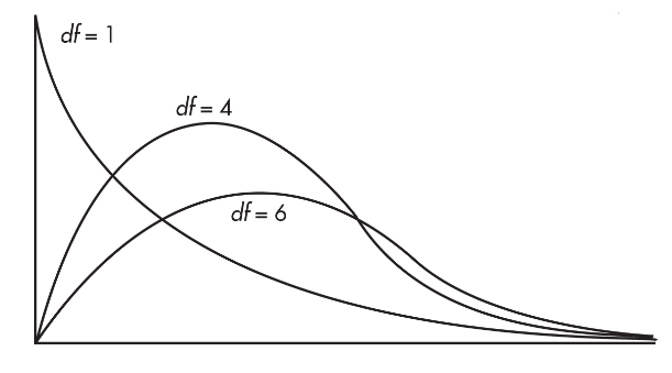
A χ2-distribution has only nonnegative values, is not symmetric, and is always skewed to the right.
There are distinct χ2-distributions, each with an associated number of degrees of freedom (df).
The larger the df value, the less pronounced is the skew, and the closer the χ2-distribution is to a normal distribution.
For inference about the distribution of a single categorical variable, such as a goodness-of-fit test, we will use a chi-square distribution with degrees of freedom, df = number of categories - 1.
➥ Example 8.1
A large city is divided into four distinct socioeconomic regions, one where the upper class lives, one for the middle class, one for the lower class, and one mixed-class region. Area percentages of the regions are 12%, 38%, 32%, and 18%, respectively. In a random sample of 55 liquor stores in the city, the numbers from each region are 4, 16, 26, and 9, respectively. The following shows how to determine if there is statistical evidence that region makes a difference with regard to numbers of liquor stores.
If liquor stores in the city were distributed among the four regions in the same proportions as the areas of those regions, what number (out of 55) would be expected in each region?
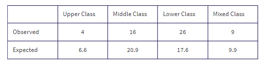
Are the sample numbers 4, 16, 26, and 9 significantly different from the expected values 6.6, 20.9, 17.6, and 9.9 to indicate that region makes a difference with regard to numbers of liquor stores?
Solution:
(0.12)(55) = 6.6, (0.38)(55) = 20.9, (0.32)(55) = 17.6, and (0.18)(55) = 9.9, and we have:
First, state the hypotheses.
H0:Liquor stores are distributed over the four city regions in the same proportions as the areas of those regions, that is, in the percentages 12, 38, 32, and 18, respectively.
Ha:Liquor stores are not distributed over the four city regions in the same proportions as the areas of those regions (at least one proportion is not as specified in the null hypothesis).
Second, name the procedure and check the conditions:
Procedure: A chi-square test for Goodness-of-fit.
Checks:
Randomization: We are given that the sample is random.
We note that the expected values (6.6, 20.9, 17.6, 9.9) are all > 5.
We assume the sample size, 55, is less than 10% of the number of all liquor stores in the large city.
Third, calculate the Χ² statistic:
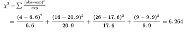
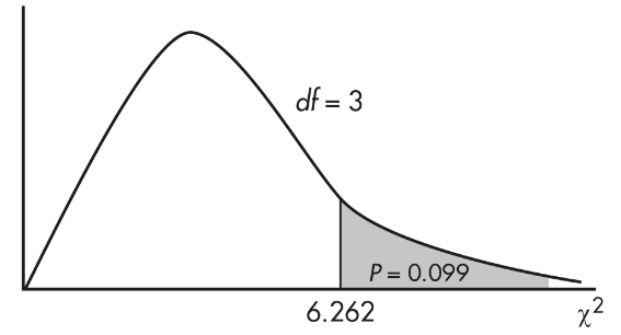
The P-value is P = P(χ2 > 6.264) = 0.099. [If n is the number of classes, df = n − 1 = 3, and χ2cdf(6.264, 1000, 3) = 0.099.] We also note that putting the observed and expected numbers in Lists, calculator software (such as χ2GOF-Test on the TI-84 or on the Casio Prizm) quickly gives χ2 = 6.262 and P = 0.099.
Fourth, give a conclusion in context with linkage to the P-value:
With this large a P-value, 0.099 > 0.05, there is not sufficient evidence to reject H0. That is, there is not convincing evidence that liquor stores in this city are distributed over the four city regions (upper, middle, lower, and mixed class) in different proportions to the areas of those regions.
Chi-Square Test for Independence
Test of Independence - There is a class of real-world problems in which we want to determine if there is a significant association between two categorical variables.
We classify our single sample observations in two ways and then ask whether the two ways are independent of each other.
For example, we might consider several age groups and within each group ask how many employees show various levels of job satisfaction. The null hypothesis is that age and job satisfaction are independent, that is, that the proportion of employees expressing a given level of job satisfaction is the same no matter which age group is considered.
When testing for independence,
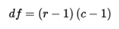
where df is the number of degrees of freedom, r is the number of rows, and c is the number of columns.
A point worth noting is that even if there is sufficient evidence to reject the null hypothesis of independence, we cannot necessarily claim any direct causal relationship.
In other words, although we can make a statement about some link or relationship between two variables, we are not justified in claiming that one causes the other.
➥ Example 8.2
A growing number of states have legalized marijuana for medical or recreational purposes. In a nationwide telephone poll of 1000 randomly selected adults representing Democrats, Republicans, and Independents, respondents were asked two questions: their party affiliation and if they supported the legalization of marijuana. The answers, cross-classified by party affiliation, are given in the following two-way table (also called a contingency table).

Test the null hypothesis that support for legalizing marijuana is independent of party affiliation. Use a 5% significance level.
Solution:
Hypothesis H0:Party affiliation and support for legalizing marijuana are independent.
Ha:Party affiliation and support for legalizing marijuana are not independent.
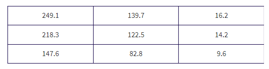
Mechanics: Putting the observed data into a "Matrix," calculator software (such as χ2-Test on the TI-84, Casio Prizm, or HP Prime) gives χ2 = 94.5 and P = 0.000, and stores the expected values in a second matrix:
Check conditions: We are given a random sample, n = 1000 is less than 10% of all adults, and we note that all expected cells are > 5.
Conclusion with linkage to the P-value: With this small of a P-value, 0.000 < 0.05, there is sufficient evidence to reject H0; that is, among all adults there is sufficient evidence of a relationship between party affiliation and support for legalizing marijuana.
Chi-Square Test for Homogeneity
Chi-square procedures can also be used with a single variable to compare samples from two or more populations.
Conditions to check include that the samples be simple random samples, that they be taken independently of each other, that the original populations be large compared to the sample sizes, and that the expected values for all cells be at least 5. The contingency table used has a row for each sample. The resulting procedure is called a chi-square test for homogeneity.
➥ Example 8.3
In a large city, a group of AP Statistics students work together on a project to determine which group of school employees has the greatest proportion who are satisfied with their jobs. In independent simple random samples of 100 teachers, 60 administrators, 45 custodians, and 55 secretaries, the numbers satisfied with their jobs were found to be 82, 38, 34, and 36, respectively. Is there evidence that the proportion of employees satisfied with their jobs is different in different school system job categories?
Solution:
Hypotheses:
H0:The proportion of employees satisfied with their jobs is the same across the various school system job categories.
Ha:At least two of the job categories differ in the proportion of employees satisfied with their jobs.
Procedure: A chi-square test for homogeneity.
Checks:
We are given independent simple random samples (a stratified random sample).
The expected cells (calculated below) are all greater than 5.
We assume that the four samples are each less than 10% of their respective populations in the large city.
Mechanics: using Matrix and χ2-Test on a calculator, we find the expected cells, the test statistic χ2, and the P-value.
The observed counts are as follows:
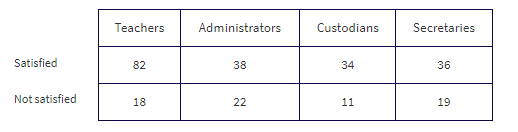
Putting the observed data into a Matrix, calculator software gives χ2 = 8.707 and P = 0.0335 and stores the expected values in a second matrix:
Conclusion in context with linkage to the P-value:
With this small of a P-value, 0.0335 < 0.05, there is sufficient evidence to reject H0; that is, there is convincing evidence that the true proportion of employees satisfied with their jobs is not the same across all the school system job categories.