Exam 2 - STATS 3110

Probability Distribution

Gives all possible events (or values) a certain variable (typically denoted by X) can product along with the probabilities for these vents/values. The variable can be quantitaitive or categorical. All probabilities must be between 0 and 1 (inclusive). All probabilities must sum to 1.

Discrete Random Variables

Have explicit corresponding probabilities. Also applies to categorical variables.

Continuous Random Variables

Can take on infinetly many values. We look at intervals instead of single values. There is no difference between ≤ and <.

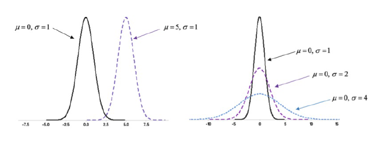
Normal Distribution

Provides a good mathematical model for many biological variables which are symmetric, such as blood pressure, bone mineral density, height of plants, weight of animals, etc. µ=0 and σ=1.

Mean (µ)

Describes the central peak around which the values are clustred (in a normal distribution)

Standard Deviation (σ)

Describes the spread of values around the mean (µ)

68-95-99.7 Rule

Data can be described by Normal distributions following this.
In the normal distribution with mean (µ) and standard deviation (σ):

• Approximately 68% of the observations fall within σ of the µ

• Approximately 95% of the observations fall within 2σ of µ

• Approximately 99.7% of the observations fall within 3σ of µ

Probability

Can be represented by the “area under the curve” and only intervals will have non-zero probability

Z-Score

Tells us how many standard deviations the observation falls from the mean in an observation. Standardizes any distribution so that it can be directly compared with others. Shows a value’s relative position within a distribution. Can also be used to find the probability of a randomly selected value falling above or below a value or between two values in the distribution.

Positive Z-Score

Indicates the observation is above the mean

Negative Z-Score

Indicates the observation is below the mean

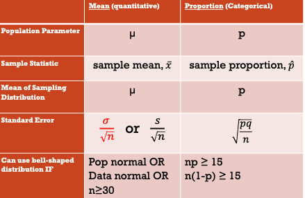
Parameter

Is a numerical value summarizing the population data (mean, median, mode, range, maximum). It is typically unknown.

Statistic

Is a numerical value summarizing the sample data (sample, mean, median, mode, range, maximum, etc.). If we have data we know and can calculate this. This can serve as estimates for population parameters.

Symbol for Sample Mean

x̄

Symbol for Population Mean

µ

Symbol for Sample Proportion

p̂

Symbol for Population Proportion

p

Symbol for Sample Standard Deviation

s

Symbol for Population Standard Deviation

σ

Symbol for Sample Variance

s²

Symbol for Population Variance

σ²

Symbol for Sample Size

n

Symbol for Population Size

N

Sampling Distribution

Is the collection of all possible sample statistics we could attain from samples of the same size from a population

Center of Sampling Distribution

Will ALWAYS be the value of the population’s parameter, regardless of sample size

Randomization and Independence Assumption

The sampled values must have been randomly selected or resulted from an experiment with random assignment, and they should be independent of each other

Sufficient Sample Size Assumption

The sample size, n, must be large enough that the sampling distribution is not truncated at either end. This is generally satisfied by the 15 successes and failures condition

Success/Failure Condition

The sample size must be big enough so that both the number of successes, np, and the number of failures, nq, are at least 15

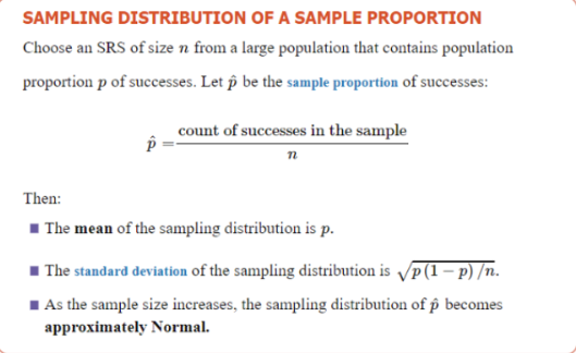
Sampling Distribution of a Sample Proportion

Standard Error

Is the standard deviation of the sampling distribution

Predicting SE using σ (the population standard deviation), then the sampling distribution for x-bar is approximately normal as long as…

• If the population has a normal distribution

• If the data (from our sample) are approximately bell-shaped, we can infer that the population from which it is drawn is also approximately bell-shaped

• For large n (n≥30), the sampling distribution of x-bar is approximately a normal distribution regardless of the distribution of the population. This is called the Central Limit Theorem (CLT)

Sample Average (x-bar)

Is a statistic with a sampling distribution of predictable shape, center, and variation

Summary of the sampling distributions

Confidence Interval

Interval estimate of a population parameter (based on the sampling distribution)

Test of Significance

Assessing the evidence for or against a claim about the population parameter (based on the sampling distribution)

“Plus Four” Adjustment

Add two observations to the number of successes and four observations to the total sample size (two successes and two failures); For large sample sizes, it makes very little difference, but this can improve the accuracy for smaller sample sizes. Use throughout the whole formula, not just SE

Changing the confidence level to a higher percentage

The interval would be wider

Pros of choosing a higher confidence level

Cons of choosing a higher confidence level

How would a smaller sample affect the width of the interval?

It would make the interval more narrow

How would a larger sample affect the width of the interval?

It would widen the interval

Hypothesis Testing

Another type of statistical inference; to determine if changes in the observed data are bigger than we would expect; provides a formal structure of testing a specific value of the population parameter, without measuring the whole population (based only on the sample results)

Hypothesis Testing Steps

1. State the hypothesis

2. Check the conditions and calculate the test statistic

3. Find the p-value

4. State the conclusion based on the context

Null Hypothesis (H₀)

Is a statement of “no effect” or “no difference”; a hypothesis test is designed to test the strength of the evidence against this (refers to the true population parameter) (not the p-hat)

• p=hypothesized value

• Never “accept” the null hypothesis; rather we speak in terms of rejecting or failing to reject

Alternative Hypothesis (Hₐ)

The more specific claim about the population that we are trying to find evidence for (refers to the true population parameter) (not the sample p-hat); the direction is determined by the comparison and will be informed by the context of the problem

• p[<,>,≠] hypothesized value

Hypothesized Value

Is the value being tested, often the value which used to be previously true

One-Sided

The alternative hypothesis is ________ if it states that a parameter is larger than or that it is smaller than the null hypothesis value

Two-Sided

It is _______ if it states that the parameter is different from the null value (it could be either smaller or larger)

Test Statistic

Measures how much evidence we have in favor of Hₐ; measures how many standard errors the current sample proportion p-hat is from the hypothesized value; it is denoted by z since it follows the standard N(0,1) distribution

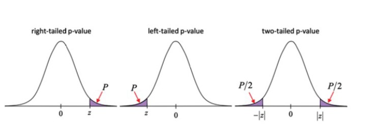
P-Value

Quantifies exactly how unlikely a particular sample proportion is; it is defined as the probability of getting a sample proportion greater or less than the current p-hat (in the direction given by Hₐ) under the assumption that H₀ is true; graphically it is the tail area of the normal distribution beyond the test statistic

Small p-value

The observation would be really unlikely if the null hypothesis were true, so we should conclude the null hypothesis is false and go with the reality presented in the alternative hypothesis

Large p-value

The observation would happen fairly often just by chance when the null hypothesis is correct, so we have no real evidence that it is wrong

Significance Level (α)

The formal cutoff between a “small” and “large” p-value

If P-value<α

Reject H₀; there is sufficient evidence to reject the null hypothesis at this significance level; there is sufficient evidence, at α, Hₐ is true

If P-value ≥ α

Fail to reject H₀; there is insufficient evidence to reject the null hypothesis at this signficance level; there is insufficient evidence, at α, Hₐ is true.

Interpretation of P-value

The chance of observing ______ (more or less) ________ in a random sample of ______ (n), if the true proportion of ________ is _______%.

Alternative hypothesis and larger sample size

Always provides greater evidence for it

Large Test Statistic

Means that in the Normal curve, the tail area beyond it becomes smaller

Larger sample size and P-value

Often, we have a higher value that is slightly above 0.05 (implying insufficient evidence of a change), taking a larger sample size might bring the P-value below 0.05 (implying sufficient evidence of a change)

• Collecting more data yielded the additional evidence to rule out randomnmess and conclude that the value has changed

Confidence interval and hypothesis testing

This can be used to predict the outcome of a two-sided hypothesis: simply check if the hypothesized value is contained inside the interval or not

If hypothesized value is outside of the confidence interval

This is clearly not a plausible value and should be rejected. That is, there is sufficient evidence to conclude the value has changed

If the hypothesized value is inside the interval

It is a plausible value and there is insufficient evidece to reject it

Hypothesis tests

__________ are not definitive proof of anything

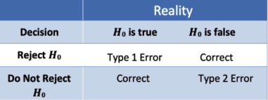
Type I Error (α)

If H₀ is really true, but we reject it (false positive)

Type II Error (β)

If Hₐ, is really true, but we continue to assume H₀ (false negative)

Error Chart

Minimizing chance of error

To decrease either Type I or Type II, you need to increase the other, or increase the sample size