Chapter 8: Confidence Intervals
Introduction
Inferential statistics: We use sample data to make generalizations about an unknown population
Sample data: help us to make an estimate of a population parameter.
Point estimate: a single number computed from a sample and used to estimate a population parameter
x¯ is a point estimate for μ
p′ is a point estimate for ρ
s is a point estimate for σ
Confidence interval: an interval estimate for an unknown population parameter. This depends on:
Confidence interval form: (point estimate – margin of error, point estimate + margin of error)
Empirical rule: Around 68% of values are within 1 standard deviation of the mean. Around 95% of values are within 2 standard deviations of the mean.
The margin of error: how many percentages points your results will differ from the real population value
8.1 A Single Population Mean using the Normal Distribution
Confidence level: considered the probability that the calculated confidence interval estimate will contain the true population parameter.
Alpha level: is the probability that the interval does not contain the unknown population parameter.
standard error of the mean: 𝜎 / √n
X¯ is normally distributed, that is, X¯~ N(𝜇𝑋 , 𝜎 / √n)
Calculating the Confidence Interval
Calculate the sample mean 𝑥⎯⎯x¯ from the sample data. Remember, in this section, we already know the population standard deviation σ.
Find the z-score that corresponds to the confidence level.
Calculate the error-bound EBM.
Construct the confidence interval.
Write a sentence that interprets the estimate in the context of the situation in the problem. (Explain what the confidence interval means, in the words of the problem.)
Finding the z-score for the Stated Confidence Level
Each of the tails contains an area equal to 𝛼/2.
The z-score that has an area to the right of 𝛼/2 is denoted by 𝑧 𝛼/2.
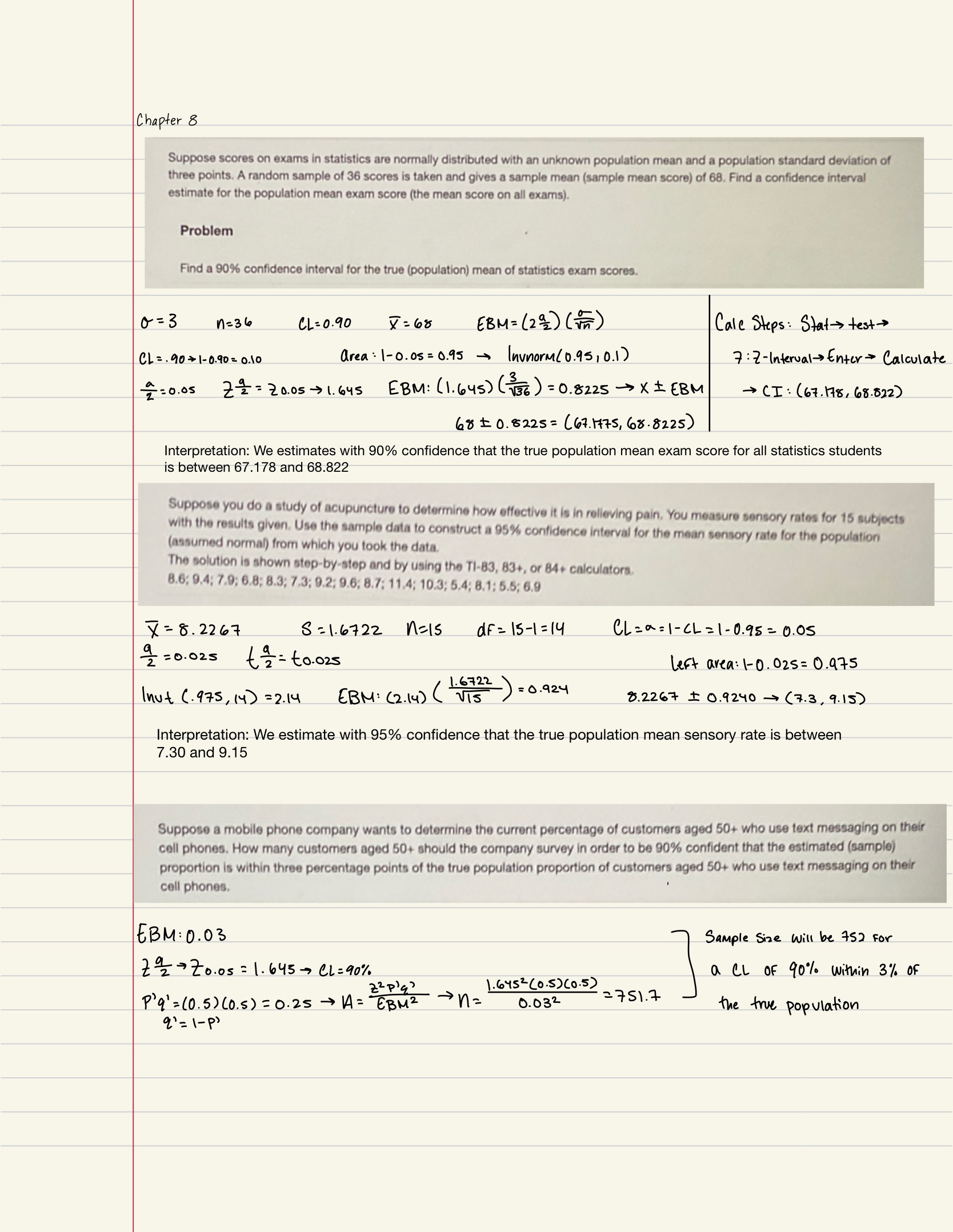
Calculating the Error Bound: EBM = (𝑧 𝛼/2)(𝜎/√n)
Confidence level interpretation: "We estimate with ___% confidence that the true population mean (include the context of the problem) is between ___ and ___ (include appropriate units)."
Effect of Changing the Confidence Level
Increasing the confidence level increases the error bound, making the confidence interval wider.
Decreasing the confidence level decreases the error bound, making the confidence interval narrower.
Effect of Changing the Sample Size
Increasing the sample size causes the error bound to decrease, making the confidence interval narrower.
Decreasing the sample size causes the error bound to increase, making the confidence interval wider.
Finding the Error Bound
From the upper value for the interval, subtract the sample mean,
OR, from the upper value for the interval, subtract the lower value. Then divide the difference by two.
Finding the Sample Mean
Subtract the error bound from the upper value of the confidence interval,
OR, average the upper and lower endpoints of the confidence interval.
8.2 A Single Population Mean using the Student t Distribution
Student's t-distribution: a type of probability distribution that is similar to the normal distribution with its bell shape but has heavier tails
Standard deviation: a number that is equal to the square root of the variance and measures how far data values are from their mean; notation: s for sample standard deviation and σ for population standard deviation
Normal distribution: continuous random variable (RV) with pdf 𝑓(𝑥)=(1 / 𝜎√2𝜋) 𝑒^–(𝑥–𝜇)^2/2𝜎^2, where μ is the mean of the distribution and σ is the standard deviation, notation: X ~ N(μ,σ).
Degrees of freedom: the number of objects in a sample that is free to vary
df = n - 1: the degrees of freedom for a Student’s t-distribution where n represents the size of the sample
The invT command requires two inputs: invT(area to the left, degrees of freedom) The output is the t-score that corresponds to the area we specified.
Properties of the Student's t-Distribution
The graph for the Student's t-distribution is similar to the standard normal curve.
The mean for the Student's t-distribution is zero and the distribution is symmetric about zero.
The Student's t-distribution has more probability in its tails than the standard normal distribution because the spread of the t-distribution is greater than the spread of the standard normal.
The exact shape of the Student's t-distribution depends on the degrees of freedom. As the degrees of freedom increase, the graph becomes more like the graph of the standard normal distribution.
The underlying population of individual observations is assumed to be normally distributed with an unknown population mean μ and unknown population standard deviation σ.
The notation for the Student's t-distribution (using T as the random variable) is:
T ~ tdf where df = n – 1.
For example, if we have a sample of size n = 20 items, then we calculate the degrees of freedom as df = n - 1 = 20 - 1 = 19 and we write the distribution as T ~ t19.
If the population standard deviation is not known, the error bound for a population mean is:
𝐸𝐵𝑀=(𝑡 𝛼/2)(𝑠√n)
𝑡𝜎2tσ2 is the t-score with area to the right equal to 𝛼2α2,
use df = n – 1 degrees of freedom, and
s = sample standard deviation.
To calculate the confidence interval directly:
Press STAT.
Arrow over to TESTS.
Arrow down to 8:TInterval and press ENTER (or just press 8).
8.3 A Population Proportion
To construct a confidence interval for a single unknown population proportion, p, we need a point estimate for p and the margin of error, E.
The sample proportion, pˆ, is the best point estimate of the population proportion, p.
The margin of r error, E, is the critical value times the standard deviation for the sample p(1 − p) proportion, z∗ (√ (p(1-p)) / n)
z∗ represents the critical value from the standard normal distribution for the confidence level desired.
Z-score formula: If 𝑃′~𝑁(𝑝 , √𝑝𝑞/𝑛) then the z-score formula is 𝑧=𝑝′−𝑝/√𝑝𝑞/𝑛
P′ follows a normal distribution for proportions:
𝑋/𝑛= 𝑃′~ 𝑁(𝑛𝑝/𝑛 , √𝑛𝑝𝑞/𝑛)
The confidence interval has the form (p′ – EBP, p′ + EBP). EBP is error bound for the proportion.
p′ = 𝑥/𝑛
p′ = the estimated proportion of successes (p′ is a point estimate for p, the true proportion.)
x = the number of successes
n = the size of the sample
Calculating the Sample Size n
If researchers desire a specific margin of error, then they can use the error-bound formula to calculate the required sample size.
The error-bound formula for a population proportion is
𝐸𝐵𝑃 = (𝑧 𝛼/2)(√𝑝′𝑞′/𝑛)
Solving for n gives you an equation for the sample size.
𝑛 = (𝑧 𝛼/2)^2 (𝑝′𝑞′) / 𝐸𝐵𝑃^2
Examples