


Chapter 2: Limits and Continuity
A. Definitions and Example
The number L is the limit of the function f(x) as x approaches c if, as the values of x get arbitrarily close (but not equal) to c, the values of f(x) approach (or equal) L.
We write: limx→cf(x)=L
In order for limx→cf(x) to exist, the values of f must tend to the same number L as x approaches c from either the left or the right.
We write limx→c−f(x) or the left-hand limit of f at c (as x approaches c through values less than c).
We write limx→c+f(x) for the right-hand limit of f at c (as x approaches c through values greater than c).
Example:
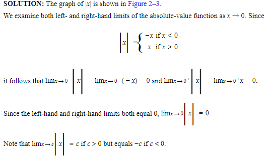
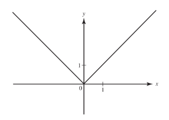
Prove that limx→0|x|=0.
SOLUTION:
Definition
The function f(x) is said to become infinite (positively or negatively) as x approaches c if f(x) can be made arbitrarily large (positively or negatively) by taking x sufficiently close to c.
We write limx→cf**(x)=+∞ (or limx→cf****(x)=−∞)**
Since, for the limit to exist, it must be a finite number, neither of the preceding limits exists.
This definition can be extended to include x approaching c from the left or from the right. The following examples illustrate these definitions.
Example:
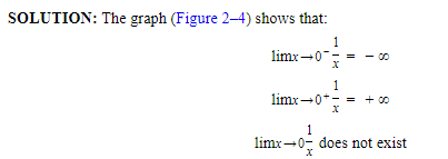
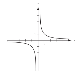
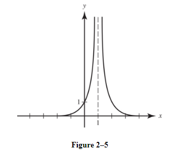
Describe the behavior of f(x)=1/x near x = 0 using limits.
SOLUTION:
Definition
We write:
limx→∞f(x)=L(or limx→−∞f(x)=L)
if the difference between f(x) and L can be made arbitrarily small by making x sufficiently large positively (or negatively).
Example:

SOLUTION:
B. Asymptotes
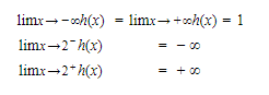
The line y = b is a horizontal asymptote of the graph of y = f(x) if limx→∞f(x)=borlimx→−∞f(x)=b.
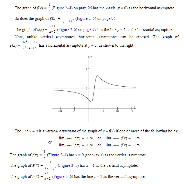
Note, unlike vertical asymptotes, horizontal asymptotes can be crossed.
Example:
SOLUTION:
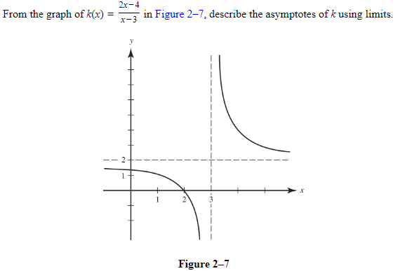
We see that y = 2 is a horizontal asymptote, since
limx→+∞k(x)=limx→−∞k(x)=2
Also, x = 3 is a vertical asymptote; the graph shows that
limx→3−k(x)=−∞ and limx→3+k(x)=+∞
C. Theorems of Limits
If B, D, E, c, and k are real numbers and if the limits of functions f and g exist at x = c such that limx→cf(x)=B and limx→cg(x)=D then:
The Constant Rule: limx→ck=k
The Constant Multiple Rule: limx→ck⋅f(x)=k⋅limx→cf(x)=k⋅B
The Sum Rule: limx→c(f(x)+g(x))=limx→cf(x)+limx→cg(x)=B+D
The Difference Rule: limx→c(f(x)−g(x))=limx→cf(x)−limx→cg(x)=B−D
The Product Rule: limx→c(f(x)⋅g(x))=limx→cf(x)⋅limx→cg(x)=B⋅D
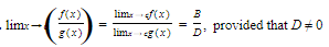
The Quotient Rule:
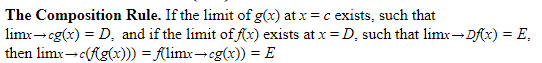
The Composition Rule:
The Squeeze or Sandwich Theorem:

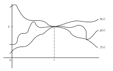
Squeezing function g between functions f and h forces g to have the same limit L at x = c as do f and g.
Example:
D. Limit of a Qoutient of Polynomials
To find

where P(x) and Q(x) are polynomials in x, we can divide both numerator and denominator by the highest power of x that occurs and use the fact that

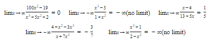
Example:
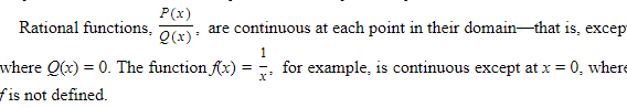
The Rational Function Theorem
This theorem holds also when we replace “x→∞” by “x→−∞.”
Note also that:
2. 
3. 
Example:
E. Other Basic Limits
E1. The basic trigonometric limit is:
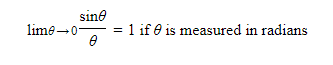
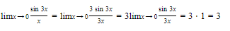
Example:

Solution:
E2. The number e can be defined as follows:
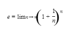
The value of e can be approximated on a graphing calculator to a large number of decimal places by evaluating
for large values of x.
F. Continuity
If a function is continuous over an interval, we can draw its graph without lifting pencil from paper. The graph has no holes, breaks, or jumps on the interval.
Conceptually, if f(x) is continuous at a point x = c, then the closer x is to c, the closer f(x) gets to f(c). This is made precise by the following definition:
Definition
The function y = f(x) is continuous at x = c if
f(c) exists (that is, c is in the domain of f)
limx→cf(x) exists
limx→cf(x)=f(c)
A function is continuous over the closed interval [a,b] if it is continuous at each x such that a ⩽ x ⩽ b.
A function that is not continuous at x = c is said to be discontinuous at that point. We then call x = c a point of discontinuity.
Continuous Functions
Polynomials are continuous everywhere—namely, at every real number.
The absolute-value function f(x) = |x|is continuous everywhere.
The trigonometric, inverse trigonometric, exponential, and logarithmic functions are continuous at each point in their domains.
Functions of the type n√x (where n is a positive integer ⩾ 2) are continuous at each x for which n√x is defined.
The greatest-integer function f(x) = [x] is discontinuous at each integer, since it does not have a limit at any integer.
Kinds of Discontinuity
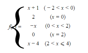
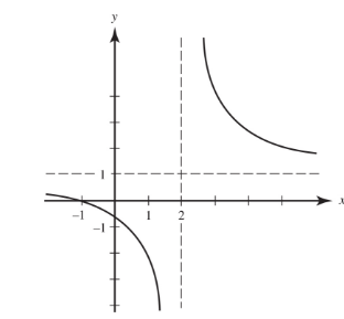
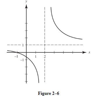
The graph of f is shown at the right.
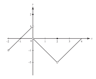
We observe that f is not continuous at x = −2, x = 0, or x = 2.
At x = −2, f is not defined.
At x = 0, f is defined; in fact, f(0) = 2.
However, since limx→0−f(x)=1 and limx→0+f(x)=0, limx→0f(x) does not exist.
Where the left- and right-hand limits exist, but are different, the function has a jump discontinuity.
The greatest-integer function, y = [x], has a jump discontinuity at every integer.
At x = 2, f is defined; in fact, f(2) = 0. Also, limx→2f(x)=−2; the limit exists.
However, limx→2f(x)≠f(2).
This discontinuity is called removable.
If we were to redefine the function at x = 2 to be f(2) = −2, the new function would no longer have a discontinuity there.
We cannot, however, “remove” a jump discontinuity by any redefinition whatsoever.
Whenever the graph of a function f(x) has the line x = a as a vertical asymptote, then f(x) becomes positively or negatively infinite as x → a+ or as x → a−.
The function is then said to have an infinite discontinuity.
Example:
 SOLUTION:
This function is continuous except where the denominator equals 0 (where g has an infinite discontinuity). It is not continuous at x = 3, but is continuous at x = 0.