Unit 7: Statistical Inference
Introduction
Parameter: characteristic of a population
Statistic: number computed from the sample
Estimation process: procedure of guessing an unknown parameter value using the observed values from samples.
Estimate: specific guess or value computed from a sample
Point estimate: a single number computed from a sample and used to estimate a population parameter
The margin of error: how many percentages points your results will differ from the real population value
Properties of a Statistic
The Center of a Statistic’s Distribution
Unbiasedness: the idea that a statistic is expected to give values centered on the unknown parameter value
Bias: the difference between the estimated probability and the true value of the parameter being estimated
The Spread of a Statistic’s Distribution
Variability: the degree of variation in statistics values.
Inefficiency: indicates that our guess is wrong unsystematically
The Confidence Interval
Confidence interval: an interval estimate for an unknown population parameter. This depends on:
Confidence interval form: (point estimate – margin of error, point estimate + margin of error)
Confidence level: considered the probability that the calculated confidence interval estimate will contain the true population parameter.
Confidence level interpretation: "We estimate with ___% confidence that the true population mean (include the context of the problem) is between ___ and ___ (include appropriate units)."
Calculator Steps
To calculate the confidence interval directly:
Press STAT.
Arrow over to TESTS.
Arrow down to 8:TInterval and press ENTER (or just press 8).
Testing a Hypothesis
Hypothesis: a statement (or claim) about a property/characteristic of a population.
Hypothesis testing: a procedure, based on sample evidence and probability, for testing claims about a property/characteristic of a population.
Null Hypothesis (H0): A statement of no change, no effect, or no difference. Assumed true until evidence indicates otherwise. We either reject or fail to reject H0.
Alternative Hypothesis (Ha): A statement that we are trying to find evidence to support; contradictory to H0.
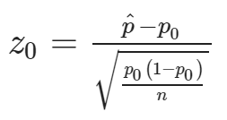
The test statistic: Measures the difference between the sample result and the null value.
p-value: the probability that, if the null hypothesis is true, the results from another randomly selected sample will be as extreme or more extreme as the results obtained from the given sample.
Large p-value: calculated from the data indicates that we should not reject the null hypothesis.
Smaller the p-value: the more unlikely the outcome, and the stronger the evidence is against the null hypothesis. We would reject the null hypothesis if the evidence is strongly against it.

Possible Errors
Type I error: We reject the null hypothesis when the null hypothesis is true. This decision would be incorrect.
α: P(Type I Error) = P(Rejecting H0 when H0 is true)
Type II error: We do not reject the null hypothesis when the alternative hypothesis is true. This decision would be incorrect.
β: P(Type II Error) = P(Failing to Reject H0 when H0 is false)
Determining the Critical Value
One-tailed tests: Left- and right-tailed tests. The alternative hypothesis changes; the null hypothesis remains the same in all three tests.
Left-tailed tests: “too small” values of the statistic as compared to the hypothesized parameter value lead to the rejection of the null hypothesis.
Right-tailed tests: “too-large” values of the statistic as compared to the hypothesized parameter a=value lead to the rejection of the null hypothesis.
The Rejection and Non-Rejection Region
Rejection or critical region (RR or CR): the set of test statistic values for which we should reject the null hypothesis
Non-rejection region: the set of test statistic values for which we should fail to reject the null hypothesis
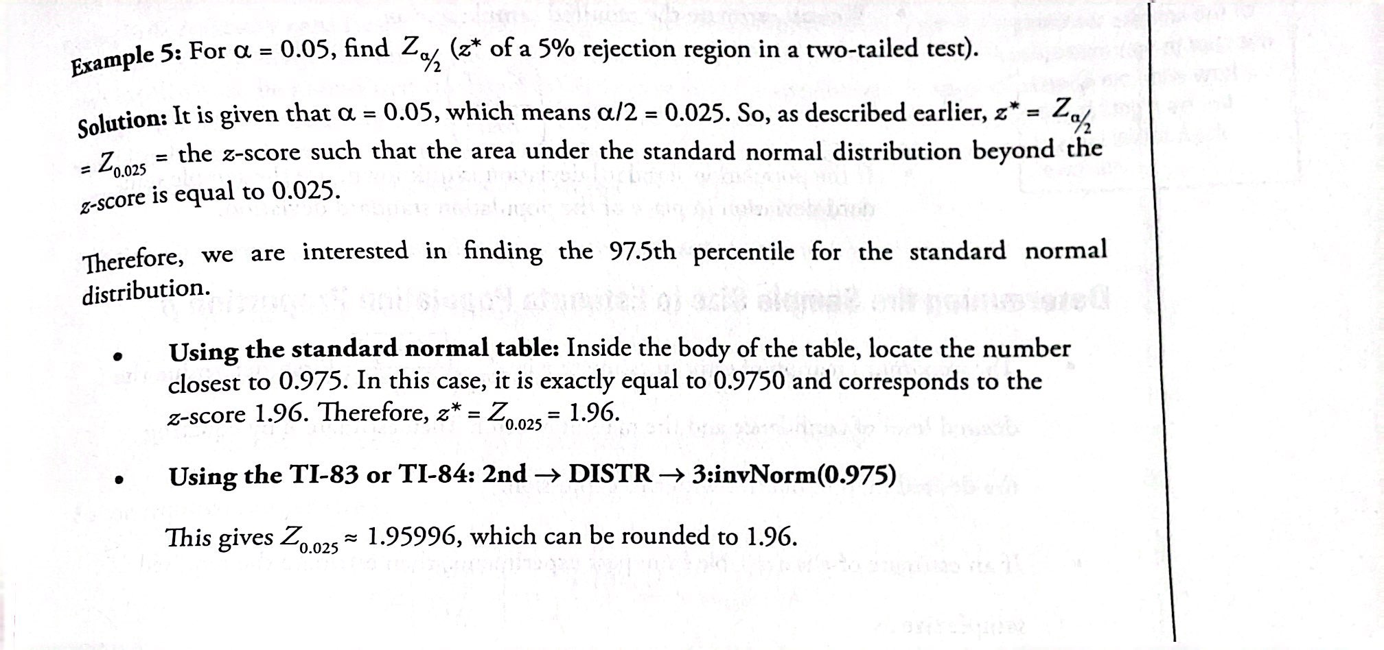
Critical value (CV): the value of a test statistic that gives the boundary between the rejection and the non-rejection region
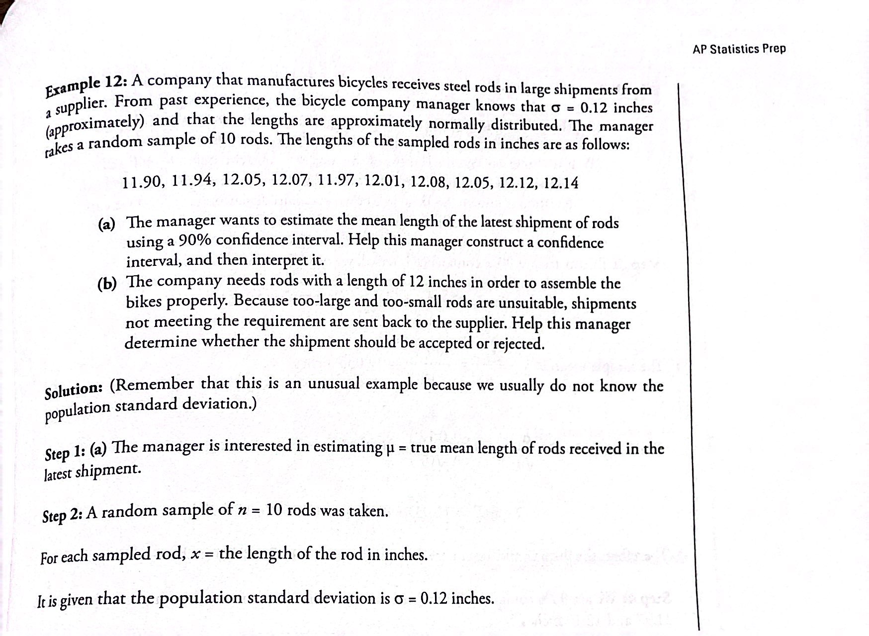
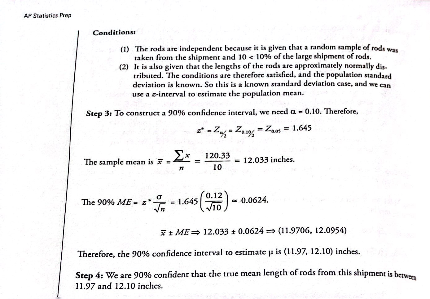
Calculating the Confidence Interval
Calculate the sample mean 𝑥⎯⎯x¯ from the sample data. Remember, in this section, we already know the population standard deviation σ.
Find the z-score that corresponds to the confidence level.
Calculate the error-bound EBM.
Construct the confidence interval.
Write a sentence that interprets the estimate in the context of the situation in the problem. (Explain what the confidence interval means, in the words of the problem.)
Acronym for proper steps to set up confidence interval→ PANIC
Parameter of interest: state what it is you are interested in with the context
Assumptions and conditions: check them fro the proper interval you are about to use
Name the type of interval: state the name of the interval that you’re about to set up
Interval: perform your calculations and set up the interval
Conclusion: conclude your results based on your interval with context
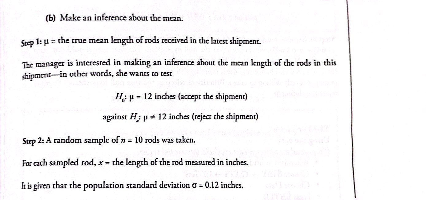
Steps for Testing a Hypothesis
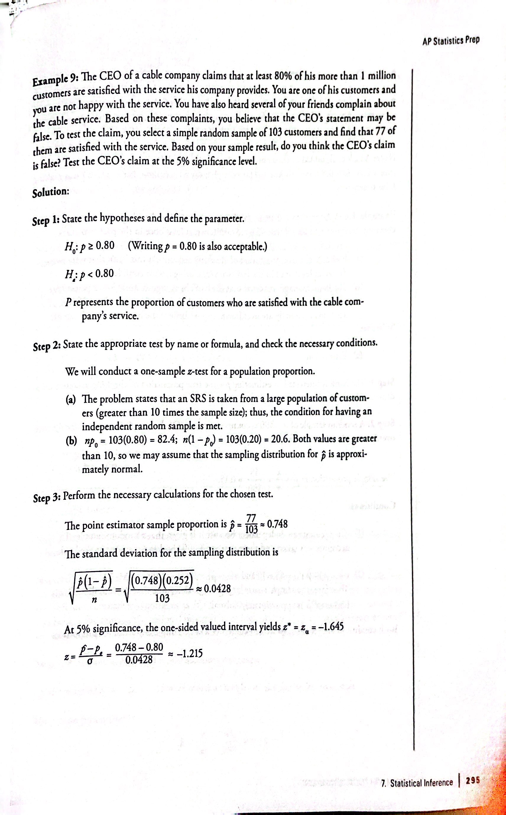
Step 1→ Determine the null and alternative hypotheses.
Step 2→ Verify all conditions have been met and state the level of significance.
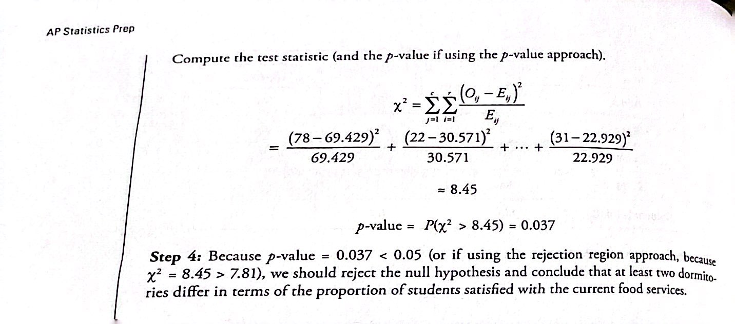
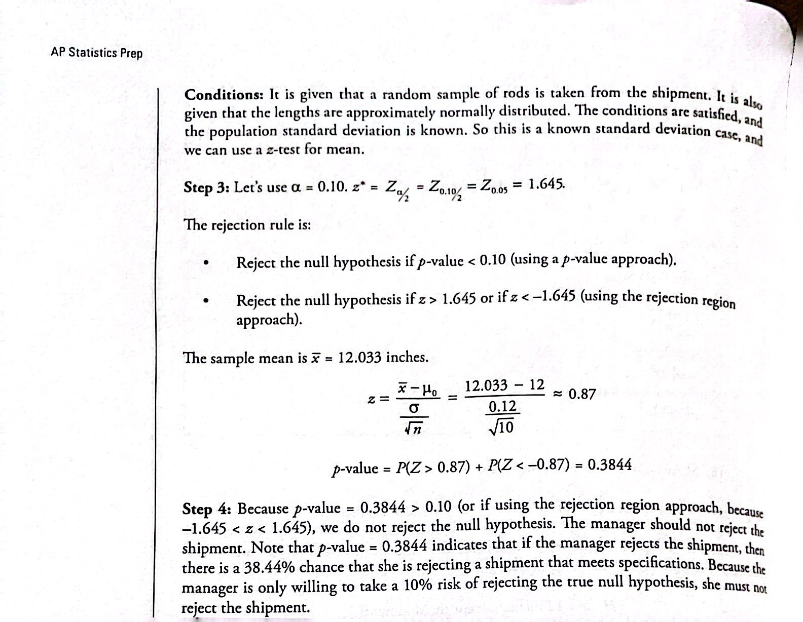
Step 3→ Summarize the data into an appropriate test statistic.
Step 4→ Find the p-value by comparing the test statistic to the possibilities expected if the null hypothesis were true OR determine the critical value.
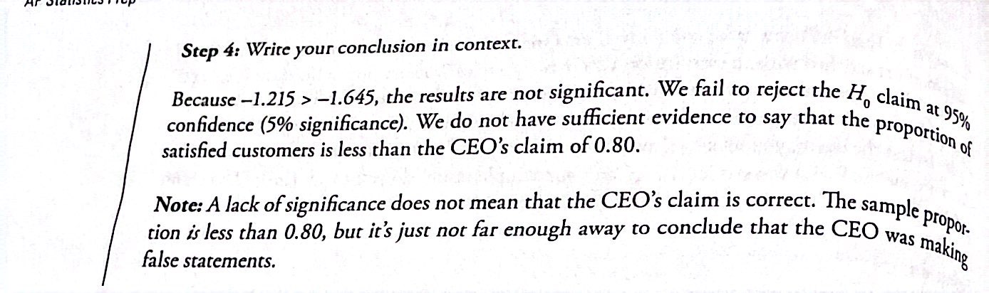
Step 5→ Decide whether the result is statistically significant based on the p-value.
p-value ≤ α: we reject the null hypothesis. (“If the P is low, the null must go!”)
p-value > α: we fail to reject the null hypothesis.
Step 6→ Report the conclusion in the context of the situation.
If you Reject H0: There is sufficient evidence to conclude [statement in Ha].
If you Fail to Reject H0: There is not sufficient evidence to conclude [statement in Ha].
Acronym for steps of hypothesis test→ PHANTOM
Parameter of interest: state what it is you are interested in with the context
Hypothesis: State your null and alternative hypothesis
Assumptions and conditions: check them for the proper test you are about to use
Name the type of test: state the name of the hypothesis test that you’re about the setup
Test statistic: perform your calculations to find the resulting test statistic
Obtain the p-value: use the test statistic you found with your sample to find the p-value
Make your decision: use your p-value to decide if you reject or fail to reject
Summarize: summarize your results based on the original question with context
Conditions
Conducting a hypothesis test that compares two independent population proportions
The two independent samples are simple random samples that are independent.
The number of successes is at least five, and the number of failures is at least five, for each of the samples.
Growing literature states that the population must be at least ten or 20 times the size of the sample.
When using a hypothesis test for matched or paired samples, the following characteristics should be present:
Simple random sampling is used.
Sample sizes are often small.
Two measurements (samples) are drawn from the same pair of individuals or objects.
Differences are calculated from the matched or paired samples.
The differences form the sample that is used for the hypothesis test.
Differences that come from a population that is normal or the number of differences is sufficiently large so that the distribution of the sample mean of differences is approximately normal.
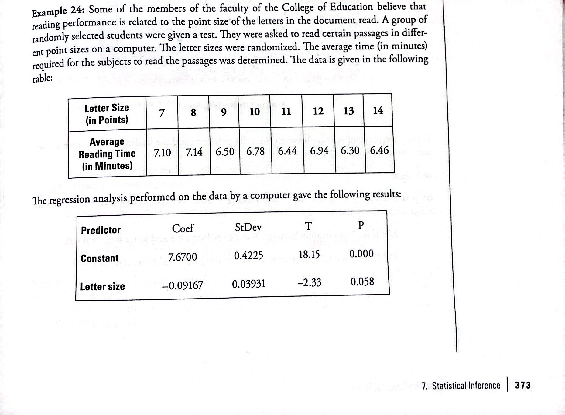
Inference for the Slope of the Least Squares Line
Least-Squares Line: You have a set of data whose scatter plot appears to "fit" a straight line
Least-squares regression line: Helps obtain a line of best fit
y0 – ŷ0 = ε0: error or residual
Absolute value of a residual: measures the vertical distance between the actual value of y and the estimated value of y
Slope equation: b = r (sy / sx)
sx = the standard deviation of the x values.
sy = the standard deviation of the y values
Interpretation of the Slope: “The slope of the best-fit line tells us how the dependent variable (y) changes for every one unit increase in the independent (x) variable, on average.”
Correlation coefficient (r): is numerical and provides a measure of strength and direction of the linear association between the independent variable x and the dependent variable y.
Using the Linear Regression T Test
In the STAT list editor, enter the X data in list L1 and the Y data in list L2, paired so that the corresponding (x,y) values are next to each other in the lists.
On the STAT TESTS menu, scroll down with the cursor to select the LinRegTTest.
On the LinRegTTest input screen enter: Xlist: L1 ; Ylist: L2 ; Freq: 1
On the next line, at the prompt β or ρ, highlight "≠ 0" and press ENTER
Leave the line for "RegEq:" blank
Highlight Calculate and press ENTER.


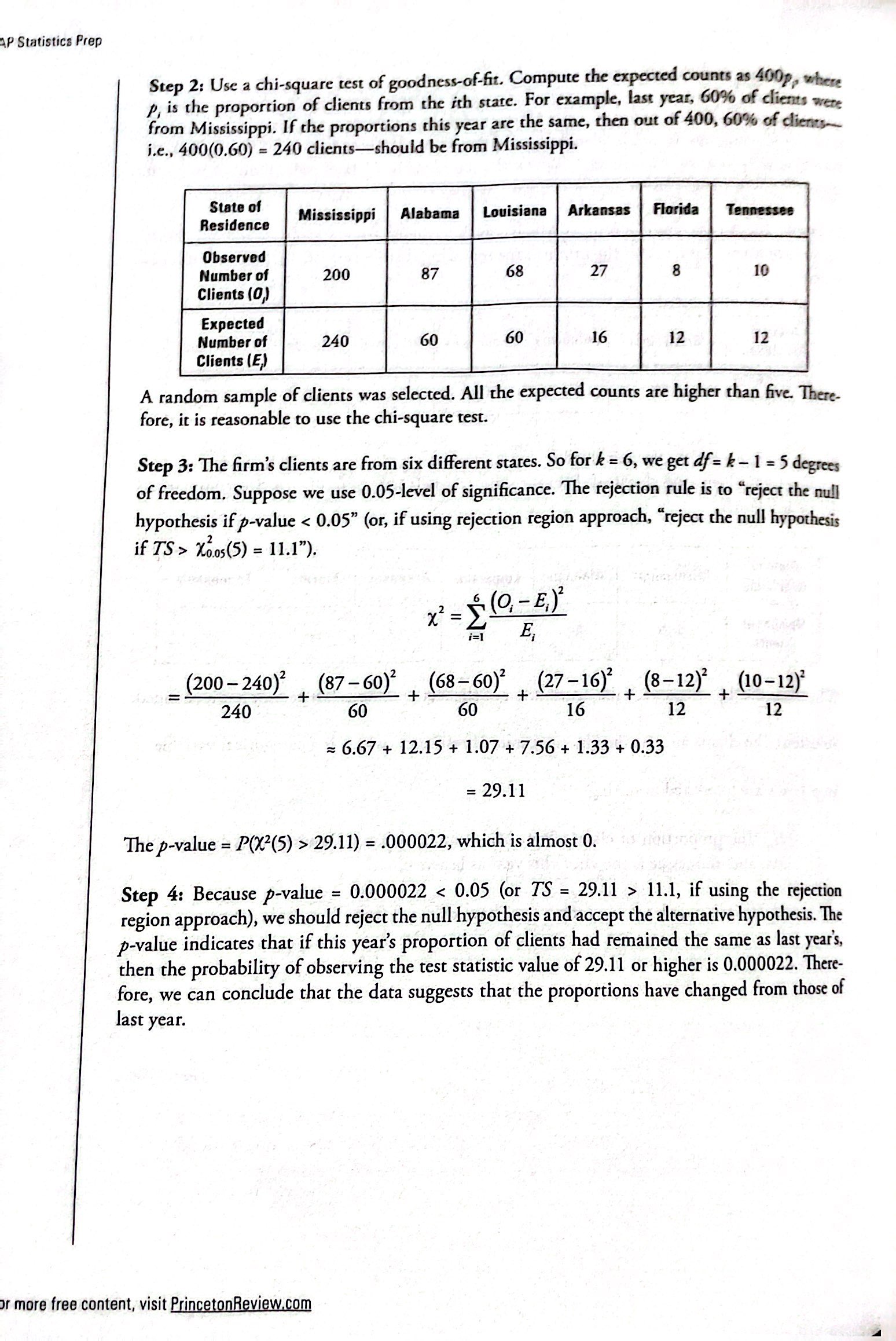
Goodness-of-Fit Test
The null and alternative hypotheses for GOF: may be written in sentences or may be stated as equations or inequalities.
Null hypothesis: The observed values of the data values and expected values are values you would expect to get.
Degrees of freedom GOF: Number of categories - 1
The goodness of fit is usually right-tailed
Large test statistic: Observed values and corresponding expected values are not close to each other.
Expected value rule: Needs to be above 5 to be able to use the test

Test of Independence
Test of independence: Determines whether two factors are independent or not
The null hypothesis for independence: states that the factors are independent
The alternative hypothesis for independence: states that they are not independent (dependent).
Independence degrees of freedom: (number of columns -1)(number of rows - 1)
Expected value formula: (row total)(column total) / total number surveyed
Test for Homogeneity
Test for Homogeneity: used to draw a conclusion about whether two populations have the same distribution
Ho: The distributions of the two populations are the same.
Ha: The distributions of the two populations are not the same.
The test statistic for Homogeneity: Use a χ2 test statistic. It is computed in the same way as the test for independence.
Chi-Square Distribution
Degrees of freedom: which depends on how chi-square is being used.
The population standard deviation is 𝜎=√2(df).
Population mean: μ = df
Comparison of the Chi-Square Test
Goodness-of-Fit: decides whether a population with an unknown distribution "fits" a known distribution.
Ho for GOF: The population fits the given distribution
Ha for GOF: The population does not fit the given distribution.
Independence: decides whether two variables are independent or dependent. There will be two qualitative variables and a contingency table will be constructed.
Ho for Independence: The two variables (factors) are independent.
Ha for Independence: The two variables (factors) are dependent.
Homogeneity: decides if two populations with unknown distributions have the same distribution as each other. There will be a single qualitative survey variable given to two different populations.
Ho of Homogeneity: The two populations follow the same distribution.
Ha of Homogeneity*:* The two populations have different distributions.