Chapter 6: Definite Integrals
A. Fundamental Theorem of Calculus (FTC); Evaluation of Definite Integral
If f is continuous on the closed interval [a,b] and F′ = f, then, according to the Fundamental Theorem of Calculus
Here ∫baf(x) is the definite integral of f from a to b; f(x) is called the integrand; and a and b are called, respectively, the lower and upper limits of integration.
This important theorem says that if f is the derivative of F then the definite integral of f gives the net change in F as x varies from a to b. It also says that we can evaluate any definite integral for which we can find an antiderivative of a continuous function.
By extension, a definite integral can be evaluated for any function that is bounded and piecewise continuous. Such functions are said to be integrable.
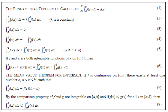
B. Properties of Definite Integrals
The following theorems about definite integrals are important.
Example:
∫2−1(3x2−2x) dx=x3−x2|2−1=(8−4)−(−1−1)=6
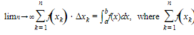
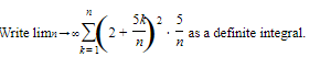
C. Definition of Definite Integral as the Limit of a Riemann Sum
This theorem provides the tool for evaluating an infinite sum by means of a definite integral.
Suppose that a function f(x) is continuous on the closed interval [a,b].
Divide the interval into n subintervals of lengths Δxk (it is not necessary that the widths be of equal length, but the formulation is generally simpler if they are).
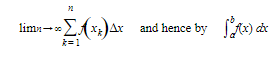
Choose numbers, one in each subinterval, as follows: x1 in the first, x2 in the second, . . ., xk in the k th, . . ., xn in the nth. Then, assuming equal width subintervals,
Δxk is called a Riemann Sum.
Example:
Solution:
D. The Fundamental Theorem Again
Area
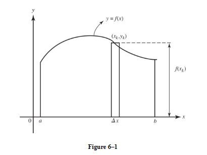
If f(x) is nonnegative on [a,b], we see (Figure 6–1) that f(xk) Δx can be regarded as the area of a typical approximating rectangle.
Assuming equal width rectangles, as the number of rectangles increases, or, equivalently, as the width Δx of the rectangles approaches zero, the rectangles become an increasingly better fit to the curve.
The sum of their areas gets closer and closer to the exact area under the curve.
Finally, the area bounded by the x-axis, the curve, and the vertical lines x = a and x = b is given exactly by
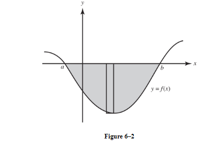
What if f(x) is negative? Then any area above the graph and below the x-axis is counted as negative (Figure 6–2).
Geometrically, area is always positive, so the shaded area above the curve and below the x-axis equals

where the integral yields a negative number. Note that every product f(xk) Δx in the shaded region is negative, since f(xk) is negative for all x between a and b.
E. Approximations of the Definite Integral; Riemann Sums
It is always possible to approximate the value of a definite integral, even when an integrand cannot be expressed in terms of elementary functions.
If f is nonnegative on [a,b], we interpret ∫b a f(x) dx as the area bounded above by y = f(x), below by the x-axis, and vertically by the lines x = a and x = b.
The value of the definite integral is then approximated by dividing the area into n strips, approximating the area of each strip by a rectangle or other geometric figure, then summing these approximations. We often divide the interval from a to b into n strips of equal width, but any strips will work.
E1. Using Rectangles
We may approximate ∫b a f(x) dx by any of the following sums, where Δx represents the subinterval widths:
(1)Left sum: f(x0) Δx1 + f(x1) Δx2 + ⋯ + f(xn − 1) Δxn, using the value of f at the left endpoint of each subinterval.
(2)Right sum: f(x1) Δx1 + f(x2) Δx2 + ⋯ + f(xn) Δxn, using the value of f at the right end of each subinterval.
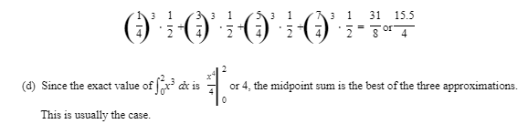
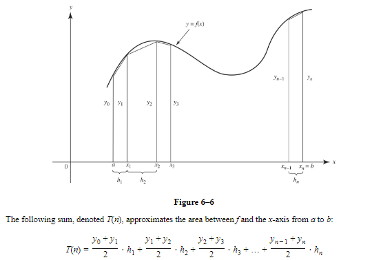
(3)Midpoint sum: 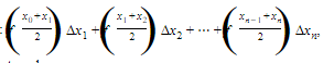
using the value of f at the midpoint of each subinterval.
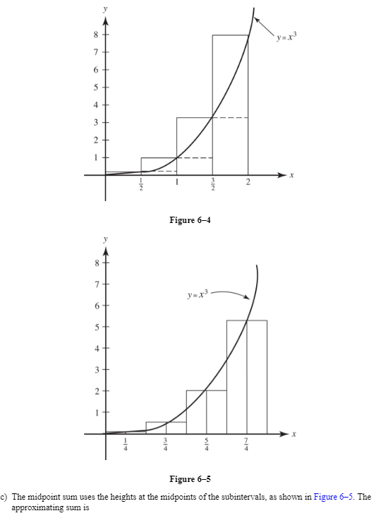
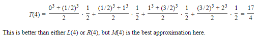
Example :
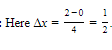
Approximate ∫20x3 dx by using four subintervals of equal width and calculating:
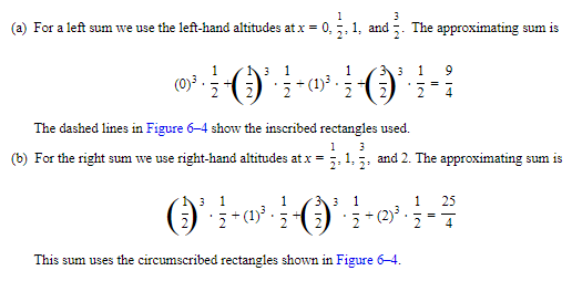
(a)the left sum
(b)the right sum
(c)the midpoint sum
(d)the integral
SOLUTIONS:
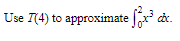
E2. Using Trapezoids
We now find the areas of the strips in Figure 6–6 by using trapezoids. We denote the bases of the trapezoids by y0*, y1, y2, . . ., yn* and the heights by Δx = h1, h2, . . ., hn.
Example:
SOLUTION:
h=12.ℎ=12. Then,
E3. Comparing Approximating Sums
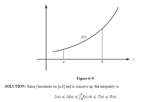
If f is an increasing function on [a,b], then L(n)⩽∫baf(x) dx⩽R(n), while if f is decreasing, then R(n)⩽∫baf(x) dx⩽L(n).
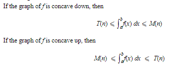
From Figure 6–7 we infer that the area of a trapezoid is less than the true area if the graph of f is concave down, but is more than the true area if the graph of f is concave up
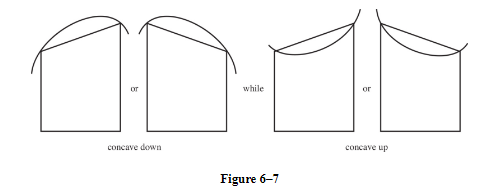
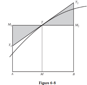
Figure 6–8 is helpful in showing how the area of a midpoint rectangle compares with that of a trapezoid and with the true area.
Our graph here is concave down. If M is the midpoint of AB, then the midpoint rectangle is AM1M2B. We’ve drawn T1T2 tangent to the curve at T (where the midpoint ordinate intersects the curve).
Since the shaded triangles have equal areas, we see that area AM1M2B = area AT1T2B. But area AT1T2B clearly exceeds the true area, as does the area of the midpoint rectangle. This fact justifies the right half of the inequality below; Figure 6–7 verifies the left half.
Generalizing to n subintervals, we conclude:
Example:
Write an inequality including L(n), R(n), M(n), T(n), and ∫baf(t) dtfor the graph of f shown in Figure 6–9.
G. Interpreting In x as an Area
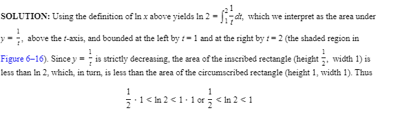
It is quite common to define ln x, the natural logarithm of x, as a definite integral, as follows:
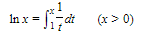
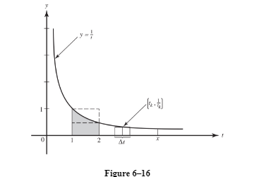
This integral can be interpreted as the area bounded above by the curve y=1t(t>0), below by the t-axis, at the left by t = 1, and at the right by t = x (x > 1).
Note that if x = 1 the above definition yields ln 1 = 0, and if 0 < x < 1 we can rewrite as follows:
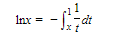
showing that ln x < 0 if 0 < x < 1.
With this definition of ln x we can approximate ln x using rectangles or trapezoids.
Example :
Show that 12<ln 2<1.12<ln 2<1.
SOLUTION:
H. Average Value
If the function y = f(x) is integrable on the interval a ⩽ x ⩽ b, then we define the average value of f from a to b to be
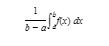
Note that (1) is equivalent to
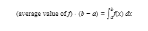
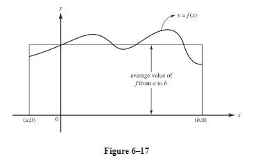
If f(x) ⩾ 0 for all x on [a,b], we can interpret (2) in terms of areas as follows:
The right-hand expression represents the area under the curve of y = f(x), above the x-axis, and bounded by the vertical lines x = a and x = b.
The left-hand expression of (2) represents the area of a rectangle with the same base (b − a) and with the average value of f as its height.
Example :
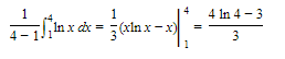
Find the average value of f(x) = ln x on the interval [1,4].
SOLUTION: