Probability

• making inferences about a population

• chance event (random phenomenon) - an activity whose outcome we can observe or measure but cannot predict the outcome for any single trial

  • each occurrence is referred to as a “success”

• probability of an event - the predicted long-run relative frequency of occurrences of that event

  • predicted proportion of “successes” → probability of success

• we can estimate probabilities experimentally and theoretically

• probability of an event must be between 0 and 1

  • 0 meaning impossible

  • 1 meaning certain

• ex) if we roll a six-sided die, how could we estimate the probability of rolling a 6?

  • experimentally: roll a die 300 times, and divide successes by total

    • if 56 were “successes” → 56/300 = 0.187

  • theoretically: assume each possible result is equally likely

    • 1/6 = 0.167

• outcome - one of the possible results of a chance process

• event - a collection of outcomes or simple events

• ex)

  • the possible outcomes for the roll of a single die are 1, 2, 3, 4, 5, and 6

  • rolling an even number: an event that consists of outcomes 2, 4, and 6

Sample Spaces and Events

• sample space - a complete list of disjoint (mutually exclusive) outcomes or events

  • disjoint - events have no outcomes in common

If we let E = event of interest, and we have defined the sample space, then the probability of E is given:

P(E) = Number of outcomes in E / Number of outcomes in the sample space

• sum of all probabilities in all possible outcomes in a sample space is 1

• 

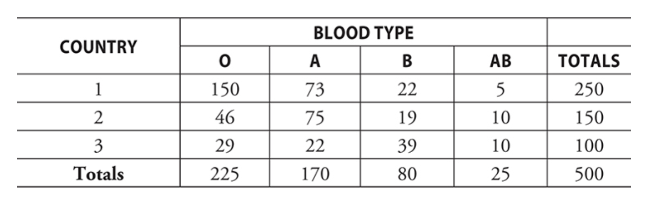
ex) Given the data above, if you randomly select a person from the population of people attending the conference, what is the probability the person has blood type A?

• P (Type A) = Number of type A / Number of people = 170/500 = 0.34

  • There is a 34% probability that a randomly selected person attending this conference has blood type A

What the rows and columns mean:

• marginal frequencies - the numbers in the total row & total colum

• joint frequencies - the cells in the middle of the table

• relative frequency - dividing a frequency in a cell by the total

  • gives the proportion of cases in that cell

  • you can also get the marginal relative frequencies & the joint relative frequencies

Probabilities of Combined Events

P (A or B) - the probability that either event A or event B occurs (or both)

• can be written as P (A ∪ B) → set notation

• spoken as “A union B”

P (A and B) - the probability that both event A and event B occur

• can be written as P (A ∩ B) → set notation

• spoken as “A intersect B”

ex) Using the same data table, if you randomly select a person from the population of people attending the conference, what is the probability the person is from Country 2 or has blood type A?

• P (Country 2 or Type A) is the sum of all joint frequencies that are either in the column for Type A or in the row for Country 2

• the cell that is in both must be counted only once

• (46 + 75 + 19 + 10) + (73 + 22) = 245 → P (Type A or Country #2) = 245/500 = 0.49

• using the addition rule:

  • add total for type A and total for Country 2, subtracting the cell that overlaps from the sum

addition rule: P (A or B) = P(A) + P(B) - P(A and B)

complement of an event A: events in the sample space that are not event A

• equal to 1 - P(A)

• denoted by Ā or A^c

ex) what is the probability that the person has blood type A, O, or AB?

• P(A, O, or AB) = 1 - P(Type B) = 1 - (420/500) = 0.84

Conditional Probability

• conditional probability - the probability of A given B

  • assumes we have knowledge of an event B having occurred before we find the probability of event A

  • denoted by P(A|B)

• 

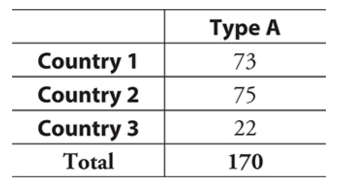
ex) if you randomly select a person with blood type A, what is the probability this person is from country 3?

• P (Country 3 | Type A) = 22/170 = 0.129

conditional probability can also be solved with a tree diagram

• tree diagram - a schematic way of looking at all possible outcomes

Independent Events

• Events A and B are said to be independent if and only if the knowledge of one event having occurred does not change the probability that the other event occurs

  • P(A|B) = P(A) or P(B|A) = P(B)

Probability of A and B or A or B

• The Multiplication Rule: P(A and B) = P(A) • P(B|A)

  • special case: if A and B are independent, P(B|A) = P(B), so P(A and B) = P(A) • P(B)

ex) if a basketball player has a 0.6 probability of making a free throw, what is his probability of making two consecutive free throws if

(a) he gets very nervous after making the first shot and his probability of making the second shot drops to 0.4?

• P(making the first shot) = 0.6

• P(making the second shot | he made the first) = 0.4.

• P(making both shots) = (0.6)(0.4) = 0.24.

(b) the events “he makes his first shot” and “he makes the succeeding shot” are independent?”

• P(he makes both shots) = (0.6)(0.6) = 0.36

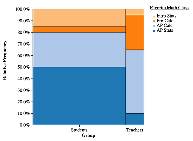
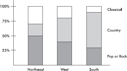
Segmented Bar Graphs and Mosaic Plots

• segmented bar graph - takes bars of equal length and equal width for each of the groups and divides them into segments that represent percentage for each category

  • need to produce conditional relative frequencies

  • 

• mosaic plot - helps preserve the relative sizes of most groups by keeping the heights the same but making widths of the bars proportional to the group size

  • 

Random Variables

• probability experiment (random phenomenon) - an activity whose outcome we can observe and measure but cannot predict the result of any single trial

• random variable X - numerical value assigned to an outcome of random phenomenon

  • P(X = x) or P(X = k) often used to show that random variable X takes on the value x

  • two types of random variables: discrete & continuous

Discrete Random Variables

• discrete random variable (DRV) - a random variable with a countable number of outcomes

  • ex) the number of successes in 20 trials of an event with a probability of success on any one trial of 0.3

Continuous Random Variables

• continuous random variable (CRV) - a random variable that takes on values associated with one or more intervals on the number line

• infinitely many outcomes within an interval

  • ex) heights of people

Probability Distribution of a Random Variable

• probability distribution for a random variable - the possible values of the random variable X together with the probabilities corresponding to those values

• probability distribution for a discrete random variable - a list of possible values of the DRV together with their respective probabilities

  • the mean (expected value) of a discrete random variable:

  • 

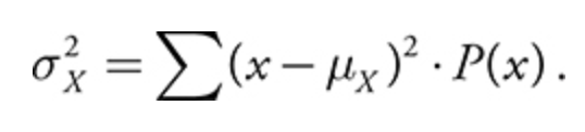
  • the variance of a discrete random variable:

  • 

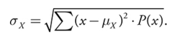
  • the standard deviation of a discrete random variable:

  • 

ex) given this probability distribution for a DRV, find P(X=3)

• since ∑Pi = 1, P(3) = 1 - (0.15 + 0.2 + 0.2 + 0.35) = 0.1

• 

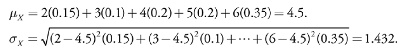
• calculator: enter x values into L1, probabilities in L2, then enter 1-var stats L1, L2

  • reads probabilities in L2 as relative frequencies and returns 4.5 for the mean and 1.432 for the standard deviation

Probability Histogram

• probability histogram - a way to picture the probability distribution

• the probability of any individual value is 0

• to find probability of an event, you must find probability that x falls in some given interval

• use the normalcdf function on your calculator

• in a normal distribution, the tails of the curve extend infinitely

  • 68-95-99.7 rule describes % of the distribution within standard deviations of the mean

  • we can standardize the normal distribution by converting to z-scores

  • 

  • a standardized normal distribution has a mean of 0 and a standard deviation of 1

Normal Probabilities

ex) in a standard normal distribution, what is the probability that z < 1.5?

• from the standard normal table, we see that the area to the left of z = 1.5 is 0.9332

  • P(z < 1.5) = 0.9332

  • 

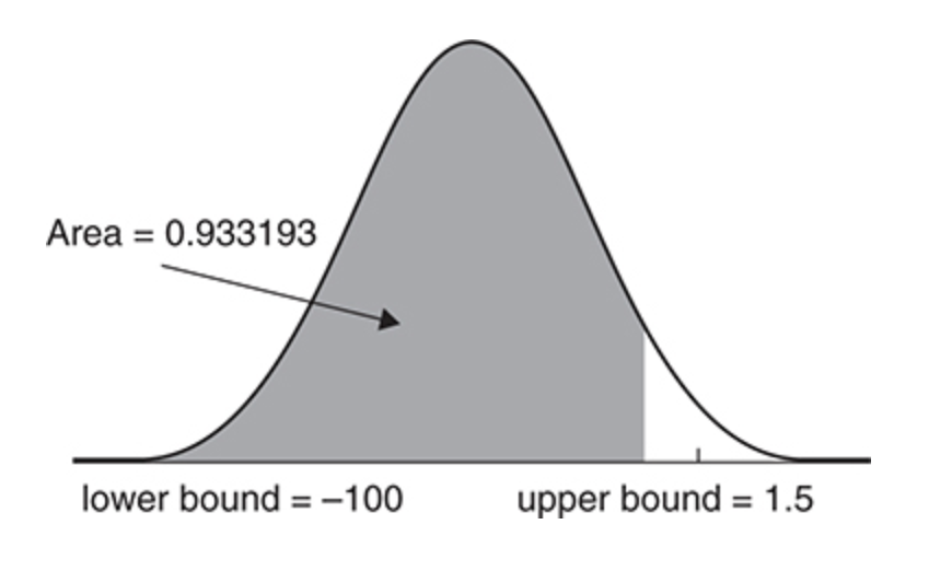
ex) the heights (X) of students at a college are normally distributed with a mean of 68 inches and a standard deviation of 3 inches, determine P(X<65)

• X ~ N (μ = 68, σ = 3)

• P(z < (65-68)/3) = -1) = 0.1597

• calculator: normalcdf (-100, -1) = normalcdf (-1000, 65, 68, 30) = 0.1586552596

ex) scores from a test are approximately normally distributed with a mean of about 500 and a standard deviation of 100. betsy needs to be in the top 15% of the test to receive a prize. what is the minimum score she must earn?

• z = (x-500)/100 = 1.04

• x = 500 + 1.04(100) = 604

• calculator: invNorm(0.85, 500, 100)

Simulation and Random Number Generation

• simulation - utilizes some random process to conduct numerous trials of the situation and then counts the number of successful outcomes to arrive at an estimated probability

• law of large numbers - the proportion of successes in the simulation should become, over time, close to the true proportion in the population

• wait-time simulation - asks how long it would take for a certain condition to occur

Transforming and Combining Random Variables

• if X is a random variable, we can transform the data by adding a constant to each value for X, multiplying each value by a constant, or a combination

Rules for the Mean and Standard Deviation of Combined Random Variables

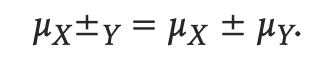
• combining means: just add

• the average of X + Y is the average for X plus the average for Y

• 

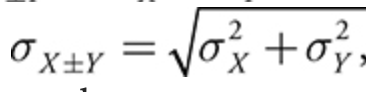
• combining variances:

  • if X and Y are independent → add

  • 

ex) a school offers an admission test. the mean score for students taking it in February (X) was 156 with a standard deviation of 12. the mean score for students taking it in March (Y) was 165 with a standard deviation of 11. what are the mean and standard deviation of the total score X + Y?

• X and Y are independent

•