Change in Tandem

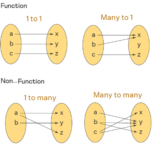
Function: a mathematical relationship that maps a set of input values to a set of output values such that each input value is mapped to exactly one output value

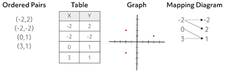
Input Values = Domain = Independent Variable (x)

Output Values = Range = Dependent Variable (y)

The input and output of a function vary according to the function rule

This can be represented graphically, verbally, analytically, or numerically

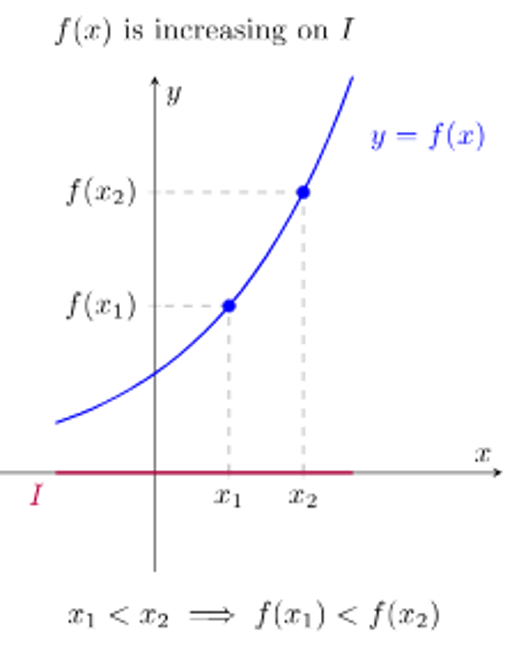
A function is increasing over an interval of its domain if:

as the input values increase, the output values always increase / for all a and b in the interval, if a < b, then f(a) < f(b)

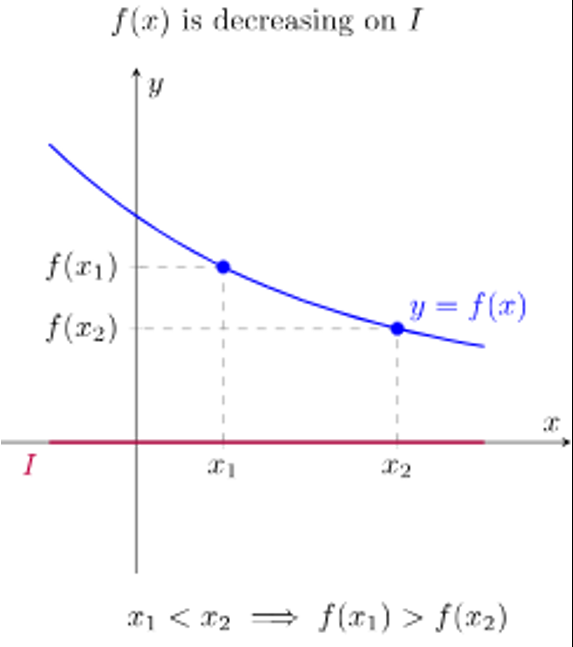
A function is decreasing over an interval of its domain if:

as the input values increase, the output values always decrease / for all a and b in the interval, if a < b, then f(a) > f(b)

Graph → a visual display of input-output pairs & shows how values vary

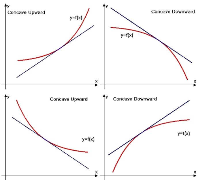
Concave up → a rate of change is increasing

Concave down → a rate of change decreasing

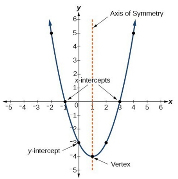
x-intercepts = zeros of the function

Rates of Change

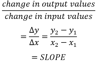
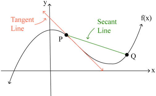
Average Rate of Change: The average rate of change over the closed interval [a, b] is the slope of the secant line from the point (a, f(a)) to (b, f(b))

The Rate of Change of a Function at a Point → approximated by the average rate of change over small intervals containing the point

Positive Rate of Change → when one quantity increases, the other quantity increases as well

Negative Rate of Change → when one quantity increases, the other quantity decreases

AROC of Linear Function → constant

•         AROC changing at a rate of 0

AROC of Quadratic Function → slope of secant line (linear)

• AROC changing at a constant rate

• If AROC is increasing over interval → concave up

• If AROC is decreasing over interval → concave down

Polynomial Functions

Polynomial Functions:

n = postitive integer                                                 polynomial degree = n

a_i = a real number for each I from 1 to n               leading term = a_nxⁿ

a_n → nonzero                                                            leading coefficient = a_n

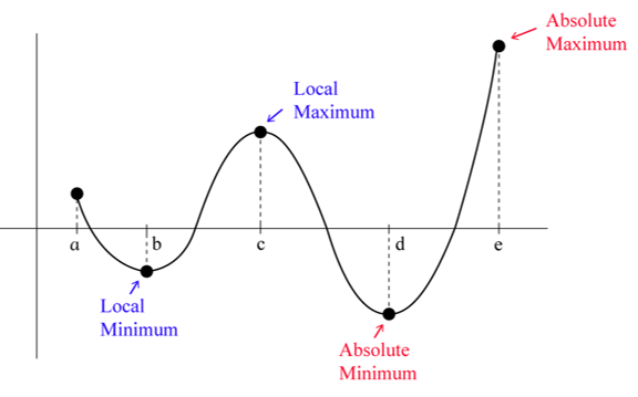
Local/Relative Maximum/Minimum: when polynomial changes between increasing and decreasing/included endpoint with restricted domain

Global/Absolute Maximum/Minimum: the greatest local maximum/least local minimum

• Between two zeros of a polynomial → at least one extrema

Points of Inflection: when rate of change of function changes from increasing to decreasing or from decreasing to increasing; changes concavity

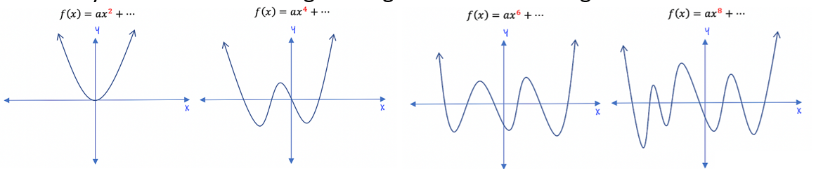
Polynomial with even degree → global maximum or global minimum

Complex Numbers: real numbers and non-real numbers

If p(a) = 0, then:

·     a → zero/root of function p

·     x-intercept at (a,0)

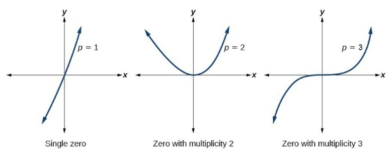
·     if a is a real number, then (x – a) is a linear factor of function p

If linear factor (x – a) is repeated n times, then there are n zeros in the functions

   └ a polynomial function of degree n has exactly n complex zeros

Real zeros of a polynomial can be endpoints for inequality intervals

If the real zero, a, has an even multiplicity (ex. (x – a)²), then the graph with “bounce” off the x-axis at x = a

Non-Real Zeros: if a + bi is a non-real zero of a polynomial p, then its conjugate a – bi is also a zero of polynomial p

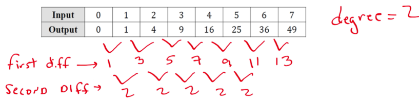
The degree of a polynomial function can be found by examining inputs and outputs of the function only if the input values are over equal intervals

  └  The degree of the function = the least value of n for which the successive nth differences are constant

Graph of even function à symmetric over the line x = 0, f(-x) = x

Even function: when n is even in polynomial of the form p(x) = a_nxⁿ*

Graph of odd function à symmetrix over the point (0, 0), f(-x) = - f(x)

Odd Function: when n is odd in polynomial of the form p(x) = a_nxⁿ*

* where n ≥ 1 and a_n­­ ≠ 0

End Behavior

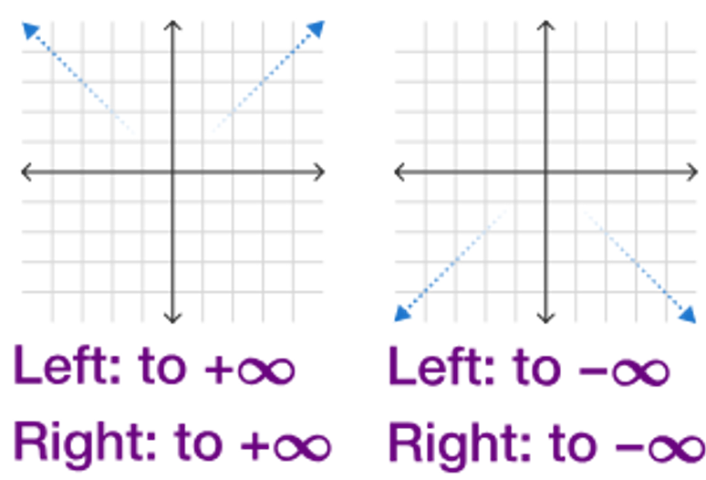
When input values of a function increase without bound, output values will either:

Increase without bound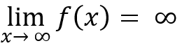

Decrease without bound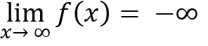

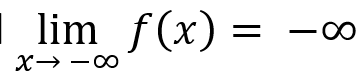
When input values of a function decrease without bound, output values will either:

Increase without bound

Decrease without bound

The degree and sign of the leading term of a polynomial determines the end behavior of the polynomial function

   └ as input values increase/decrease without bound, the values of the leading term dominate

Rational Function

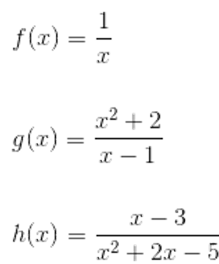
Rational Function: the ratio of two polynomials where the polynomial in the denominator ≠ 0

end behavior → affected by the polynomial of greater degree (values will dominate); can be understood by examining quotient of polynomial leading terms

ex.              

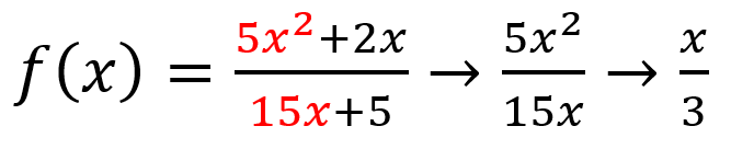x grows as at a faster rate than 3, so function will go to ∞

-if numerator dominates → quotient of leading terms is nonconstant polynomial à og function shares same end behavior

   └ if leading term polynomial is linear → graph of rational function has slant asymptote parallel to the the graph of the line

-if denominator dominates → quotient of leading terms is (constant)/(nonconstant polynomial) à graph of og function has horizontal asymptote as y = 0

-if neither dominates → quotient of leading terms is constant = horizontal asymptote of og function

Rational Function Real Zeros → real zeros of the numerator in domain

   └ real zeros of both polynomials in rational function are endpoints/asymptotes for intervals satisfying the inequalities r(x)≥ 0 or r(x) ≤ 0

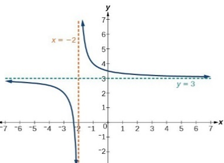
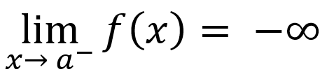
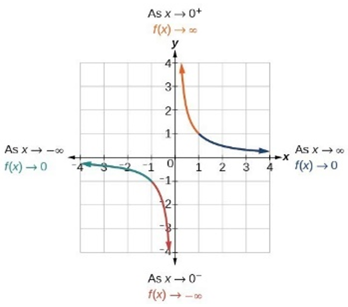
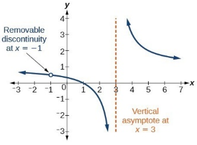
Vertical Asymptote → zeros of the polynomial in the denominator (and not numerator) / the zero appears more times in the denominator than in the numerator

Ex.   

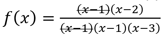since (x – 1) appears more times in the denominator, it would be a vertical asymptote

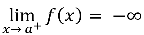
If input values are greater than asymptote, then

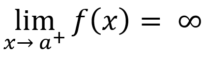or

If input values are less than asymptote, then

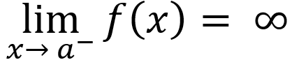or

Hole → when a zero appears more times in the numerator than the denominator

-Find the location of the hole by plugging in zero value into function

Equivalent Representations of Polynomial and Rational Expressions

standard form of polynomial and rational functions à used to find end behavior

factored form of polynomial and rational functions à used to find x-intercepts, asymptotes, holes, domain, and range

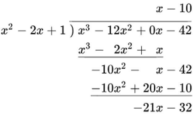
Polynomial Long Division à used to find equations of slant asymptotes of graphs of rational functions

  └ degree of remainder is less that degree of divider

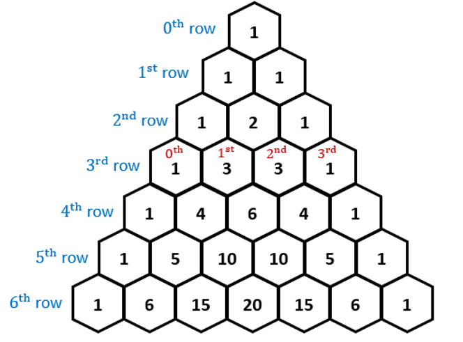
Binomial Theorem → used to expand terms in the form (a + b)ⁿ and polynomials functions in the form of (x + c)ⁿ (where c is a constant) by using Pascal’s Triangle

Ex.

Pascal’s Triangle:

Transformations of Functions

Functions can be transformed from parent function f(x)

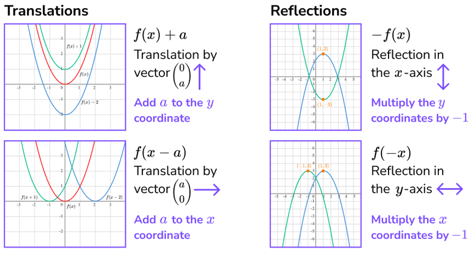
g(x) = f(x) + k  → vertical transformation of f(x) by k units

g(x) = f(x + h) → horizontal transformation of f(x) by -h units

g(x) = a f(x), where a ≠ 0 → vertical dilation by a factor of |a|;

 if a < 0 → reflection over the x-axis

g(x) = f(bx), where b ≠ 0 → horizontal dilation by a factor of |  |, if b < 0 → reflection over y-axis

*The domain and range of a transformed function may differ from the parent function

Function Model Selection and Assumption Articulation

Linear Functions → used for contextual scenarios with roughly constant rates of change

Quadratic Functions → used for contextual scenarios with roughly linear rates of change/ roughly symmetrical data sets with a unique minimum/maximum value

Geometric → used for contextual scenarios involving area/volume; two dimensions modeled by quadratic functions, three dimensions modeled by cubic functions.

Polynomial → used to model data sets/scenarios with multiple zeros or multiple extremas

Piece-wise → a set of functions defined over nonoverlapping domain interval; used for data sets/contextual scenarios that have different characteristics over different intervals

Assumptions and Restrictions of Function Model

a model may:

-assume what is consistent

-how quantities change together

-require domain restrictions (based on mathematical clues, context clues and/or extreme values)

-require range restrictions (ex. rounding values) (based on mathematical clues, context clues and/or extreme values)

Function Model Construction and Application

A model can be constructed in multiple ways:

- based on restrictions from a scenario

- using transformations from the parent function

- technology and regressions (linear, quadratic, cubic, & quartic)

- a piece-wise function can be constructed through a combination of the techniques above

Data sets that have quantities that are inversely proportional → rational functions

Ex.

Application:

Models can be used to draw conclusions about the data set/scenario

Appropriate units of measure should be used when given