

AP Precalculus Ultimate Guide
Unit 1: Polynomial and Rational Functions Flashcards
Change in Tandem
Function: a mathematical relationship that maps a set of input values to a set of output values such that each input value is mapped to exactly one output value
Input Values = Domain = Independent Variable (x)
Output Values = Range = Dependent Variable (y)
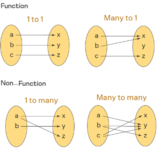
The input and output of a function vary according to the function rule
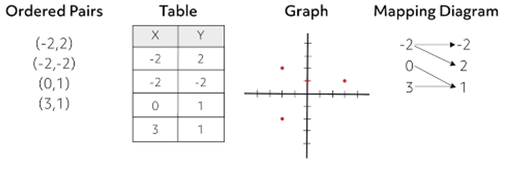
This can be represented graphically, verbally, analytically, or numerically
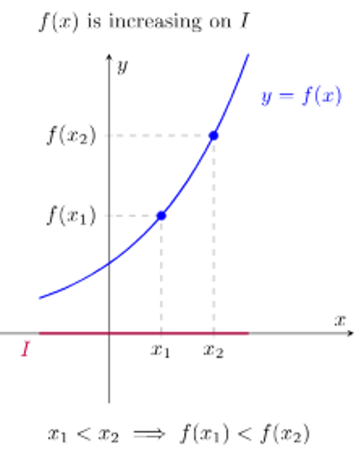
A function is increasing over an interval of its domain if:
as the input values increase, the output values always increase / for all a and b in the interval, if a < b, then f(a) < f(b)
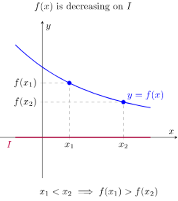
A function is decreasing over an interval of its domain if:
as the input values increase, the output values always decrease / for all a and b in the interval, if a < b, then f(a) > f(b)
Graph → a visual display of input-output pairs & shows how values vary
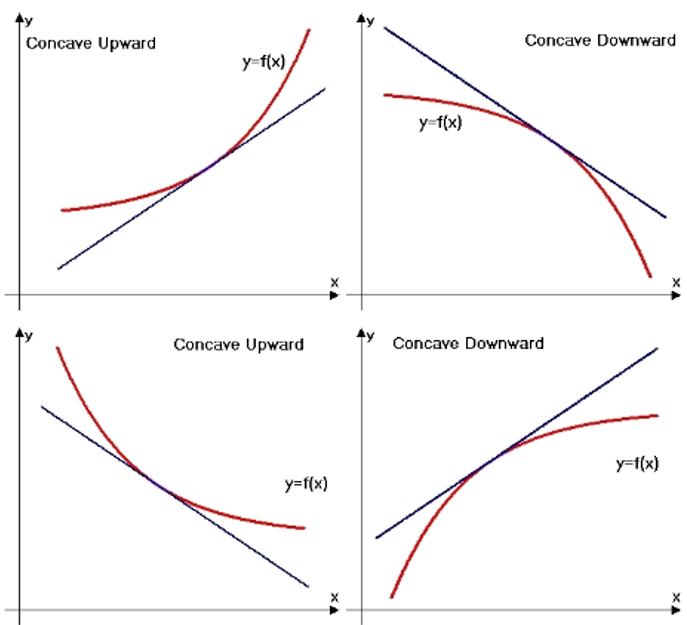
Concave up → a rate of change is increasing
Concave down → a rate of change decreasing
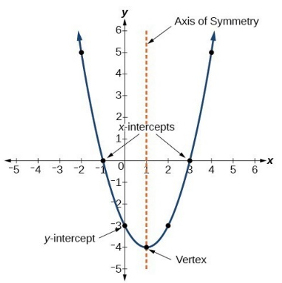
x-intercepts = zeros of the function
Rates of Change
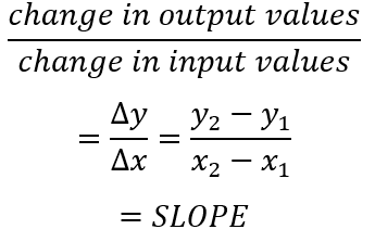
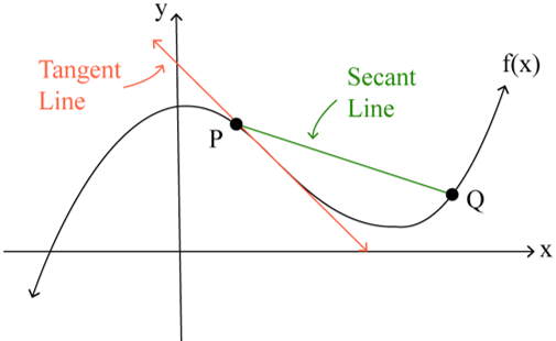
Average Rate of Change: The average rate of change over the closed interval [a, b] is the slope of the secant line from the point (a, f(a)) to (b, f(b))
The Rate of Change of a Function at a Point → approximated by the average rate of change over small intervals containing the point
Positive Rate of Change → when one quantity increases, the other quantity increases as well
Negative Rate of Change → when one quantity increases, the other quantity decreases
AROC of Linear Function → constant
AROC changing at a rate of 0
AROC of Quadratic Function → slope of secant line (linear)
AROC changing at a constant rate
If AROC is increasing over interval → concave up
If AROC is decreasing over interval → concave down
Polynomial Functions
Polynomial Functions:

n = postitive integer polynomial degree = n
ai = a real number for each I from 1 to n leading term = anxn
an → nonzero leading coefficient = an
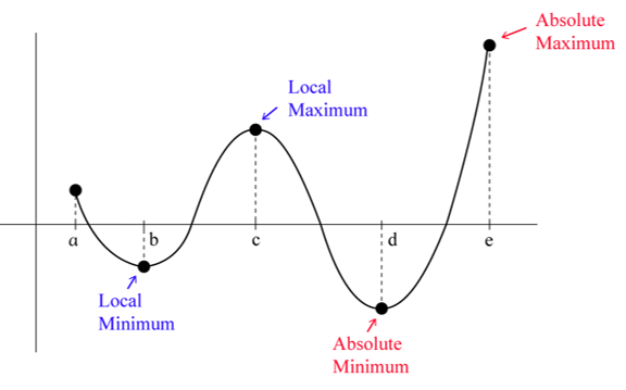
Local/Relative Maximum/Minimum: when polynomial changes between increasing and decreasing/included endpoint with restricted domain
Global/Absolute Maximum/Minimum: the greatest local maximum/least local minimum
Between two zeros of a polynomial → at least one extrema
Points of Inflection: when rate of change of function changes from increasing to decreasing or from decreasing to increasing; changes concavity
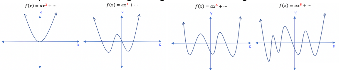
Polynomial with even degree → global maximum or global minimum
Complex Numbers: real numbers and non-real numbers
If p(a) = 0, then:
a → zero/root of function p
x-intercept at (a,0)
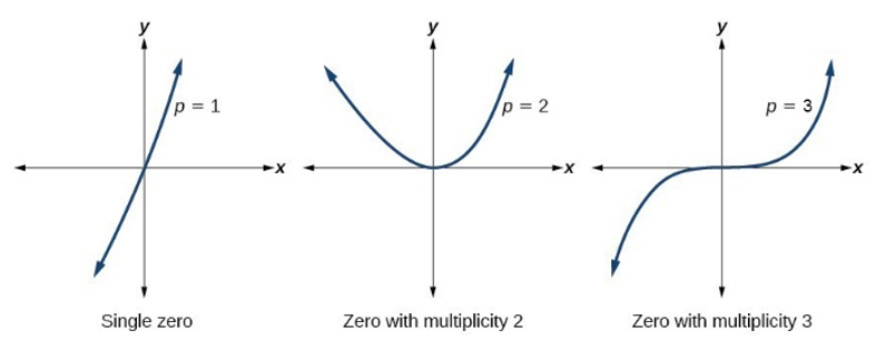
if a is a real number, then (x – a) is a linear factor of function p
If linear factor (x – a) is repeated n times, then there are n zeros in the functions
└ a polynomial function of degree n has exactly n complex zeros
Real zeros of a polynomial can be endpoints for inequality intervals
If the real zero, a, has an even multiplicity (ex. (x – a)2), then the graph with “bounce” off the x-axis at x = a
Non-Real Zeros: if a + bi is a non-real zero of a polynomial p, then its conjugate a – bi is also a zero of polynomial p
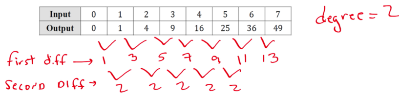
The degree of a polynomial function can be found by examining inputs and outputs of the function only if the input values are over equal intervals
└ The degree of the function = the least value of n for which the successive nth differences are constant
Graph of even function à symmetric over the line x = 0, f(-x) = x
Even function: when n is even in polynomial of the form p(x) = anxn*
Graph of odd function à symmetrix over the point (0, 0), f(-x) = - f(x)
Odd Function: when n is odd in polynomial of the form p(x) = anxn*
* where n ≥ 1 and an ≠ 0
End Behavior
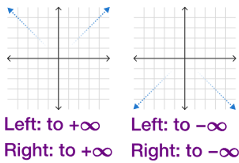
When input values of a function increase without bound, output values will either:
Increase without bound 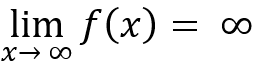
Decrease without bound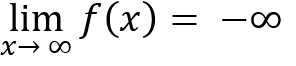
When input values of a function decrease without bound, output values will either:
Increase without bound
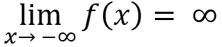
Decrease without bound
The degree and sign of the leading term of a polynomial determines the end behavior of the polynomial function
└ as input values increase/decrease without bound, the values of the leading term dominate
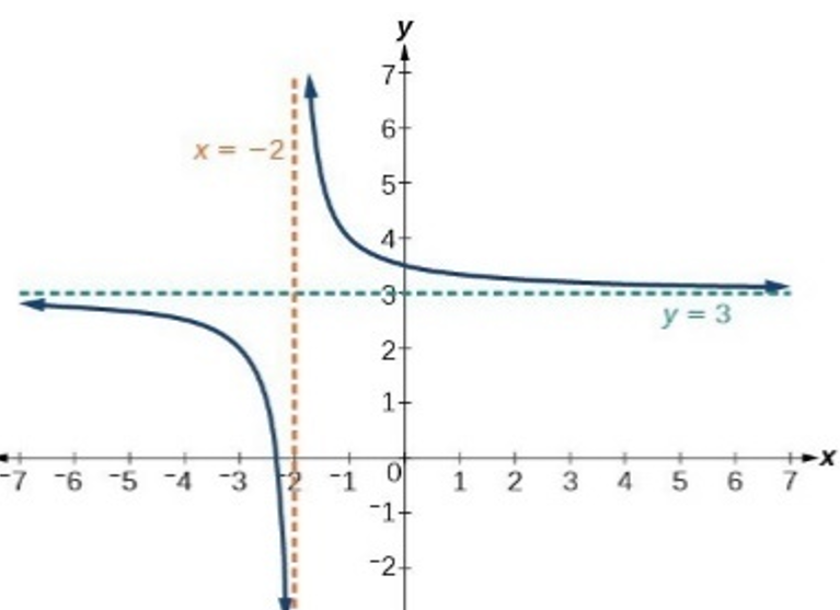
Rational Function
Rational Function: the ratio of two polynomials where the polynomial in the denominator ≠ 0
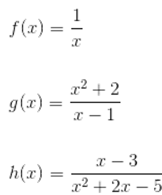
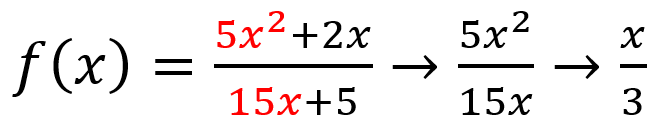
end behavior → affected by the polynomial of greater degree (values will dominate); can be understood by examining quotient of polynomial leading terms
ex.
 x grows as at a faster rate than 3, so function will go to ∞
-if numerator dominates → quotient of leading terms is nonconstant polynomial à og function shares same end behavior
└ if leading term polynomial is linear → graph of rational function has slant asymptote parallel to the the graph of the line
-if denominator dominates → quotient of leading terms is (constant)/(nonconstant polynomial) à graph of og function has horizontal asymptote as y = 0
-if neither dominates → quotient of leading terms is constant = horizontal asymptote of og function
Rational Function Real Zeros → real zeros of the numerator in domain
└ real zeros of both polynomials in rational function are endpoints/asymptotes for intervals satisfying the inequalities r(x)≥ 0 or r(x) ≤ 0
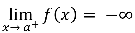
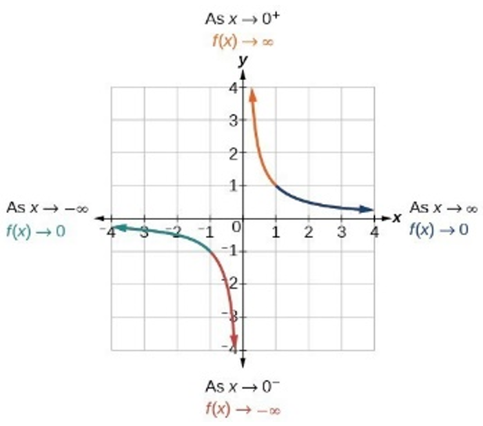
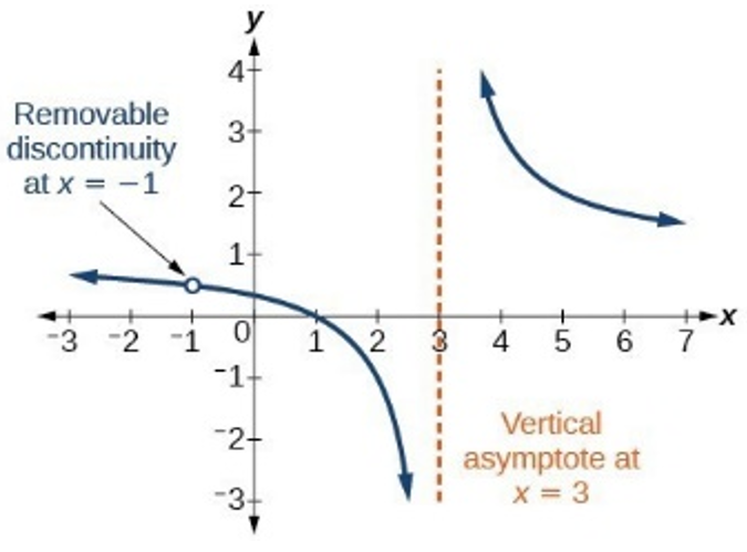
Vertical Asymptote → zeros of the polynomial in the denominator (and not numerator) / the zero appears more times in the denominator than in the numerator
Ex.
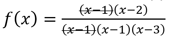 since (x – 1) appears more times in the denominator, it would be a vertical asymptote
If input values are greater than asymptote, then
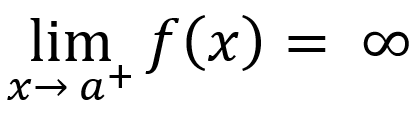 or
or
If input values are less than asymptote, then
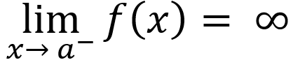 or
or
Hole → when a zero appears more times in the numerator than the denominator
-Find the location of the hole by plugging in zero value into function
Equivalent Representations of Polynomial and Rational Expressions
standard form of polynomial and rational functions à used to find end behavior
factored form of polynomial and rational functions à used to find x-intercepts, asymptotes, holes, domain, and range
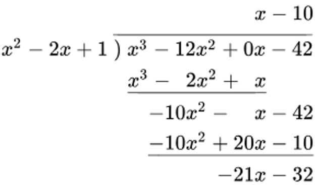
Polynomial Long Division à used to find equations of slant asymptotes of graphs of rational functions
└ degree of remainder is less that degree of divider
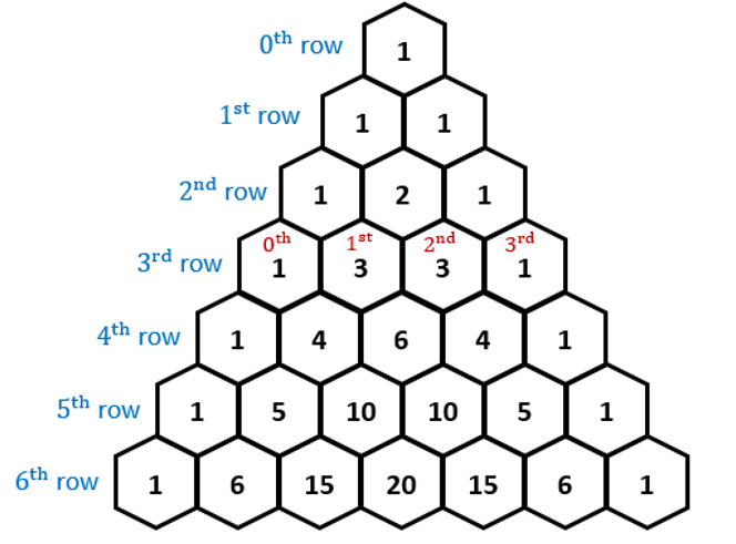
Binomial Theorem → used to expand terms in the form (a + b)n and polynomials functions in the form of (x + c)n (where c is a constant) by using Pascal’s Triangle
Ex.

Pascal’s Triangle:
Transformations of Functions
Functions can be transformed from parent function f(x)
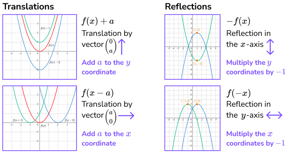
g(x) = f(x) + k → vertical transformation of f(x) by k units
g(x) = f(x + h) → horizontal transformation of f(x) by -h units
g(x) = a f(x), where a ≠ 0 → vertical dilation by a factor of |a|;
if a < 0 → reflection over the x-axis
g(x) = f(bx), where b ≠ 0 → horizontal dilation by a factor of | |, if b < 0 → reflection over y-axis
*The domain and range of a transformed function may differ from the parent function
Function Model Selection and Assumption Articulation
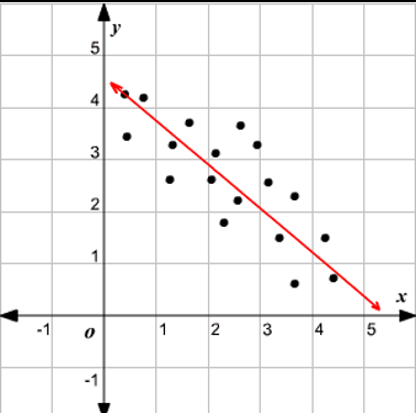
Linear Functions → used for contextual scenarios with roughly constant rates of change
Quadratic Functions → used for contextual scenarios with roughly linear rates of change/ roughly symmetrical data sets with a unique minimum/maximum value
Geometric → used for contextual scenarios involving area/volume; two dimensions modeled by quadratic functions, three dimensions modeled by cubic functions.
Polynomial → used to model data sets/scenarios with multiple zeros or multiple extremas
Piece-wise → a set of functions defined over nonoverlapping domain interval; used for data sets/contextual scenarios that have different characteristics over different intervals
Assumptions and Restrictions of Function Model
a model may:
-assume what is consistent
-how quantities change together
-require domain restrictions (based on mathematical clues, context clues and/or extreme values)
-require range restrictions (ex. rounding values) (based on mathematical clues, context clues and/or extreme values)
Function Model Construction and Application
A model can be constructed in multiple ways:
- based on restrictions from a scenario
- using transformations from the parent function
- technology and regressions (linear, quadratic, cubic, & quartic)
- a piece-wise function can be constructed through a combination of the techniques above
Data sets that have quantities that are inversely proportional → rational functions
Ex.
Application:
Models can be used to draw conclusions about the data set/scenario
Appropriate units of measure should be used when given
Unit 2: Exponential and Logarithmic Functions Flashcards
Arithmetic and Geometric Sequences
Sequence: an ordered list of numbers, with each listed number being a term. It could be finite or infinite
Arithmetic Sequence: when each successive term in a sequence has a common difference (constant rate of change)
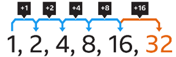
Geometric Sequence: when each successive term in a sequence has a common ratio (consistent proportional change)
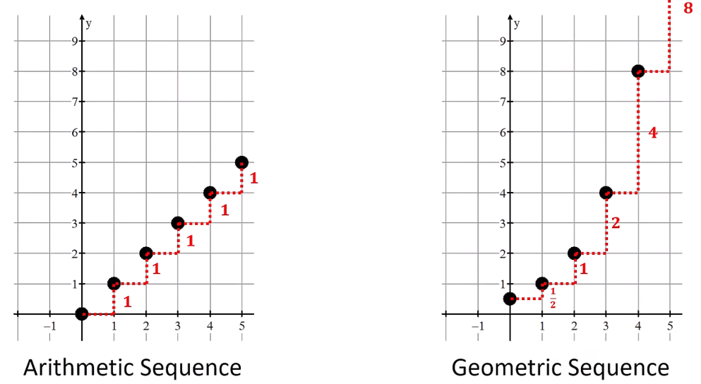
Over equal-length input-value intervals, if the output values of a function change:
at a constant rate → linear function (addition)
at a proportional rate → exponential function (multiplication)
^ all can be determined by two distinct sequence or function values
nth term (arithmetic): an = a0 + dn a0 = initial value (zero term) d = common difference (similar to slope-intercept form) |
nth term using any term (arithmetic): an = ak + d (n – k) ak = kth term of the sequence (similar to point-slope form) |
nth term (geometric): gn = g0rn g0 = initial value (zero term) r = common ratio (similar to exponential function) |
nth term using any term (geometric): gn = gk ∙ r(n – k) gk = kth term of the sequence (similar to shifted exponential) |
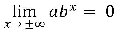
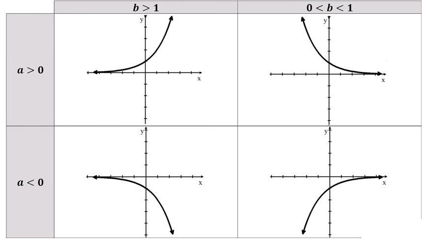
Exponential Functions f(x) = bx
-are always increasing or always decreasing
└ no extrema except on a closed interval
-always concave up or always concave down
└ no inflection points
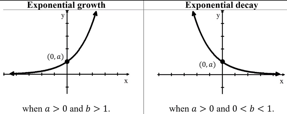
-if input values increase/decrease without bound, end behavior:
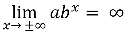 or
or
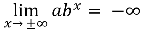 or
or
Horizontal Translation/Vertical Dialation: f(x) = b(x+k) = bx ∙ bk = abx where a = bk
Horizontal Dialation: f(x) = b(cx) → change of the base of function bc is a constant and c ≠ 0
Exponential functions model growth patterns with successive output values over equal-length input-values intervals are proportional
A constant may need to be added to the dependent variables of a data set to see proportional growth pattern
An exponential function can be constructed from: a ratio and initial value/two input-output pairs
base of exponent (b) → growth factor in successive unite changes in input values; percent change in context
forms of exponential functions can be used in different scenarios:
ex. if d = number of days f(x) = 2d → quantity increases by factor of 2 every day
f(x) = (27)(d/7) → quantity increase by a factor of 27 every 7 days/week
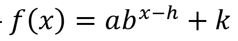
General Form of an Exponential Function: An exponential function has the general form f(x) = abx a = initial value ≠ 0 b > 0 |
Additive Transformation of an Exponential Function: g(x) = f(x) + k If the output values of g are proportional over equal-length input-value intervals, then f(x) is exponential |
Negative Exponent Property: b-n = (1/bn) |
Product Property: bmbn = b(m+n) |
Power Property: (bm)n = bmn |
The number e: e = 2.718… the natural base e is often used as the base in exponential functions |
Competing Function Model Validation
Model can be an appropriation for data if data set/regression is without pattern
Predicted vs actual results → error in model
May be appropriate to overestimate/underestimate for given interval
Composition of Functions
(f ⸰ g)(x)/f(g(x)) à maps set of input values to set of output values such that the output values of g are used as input values of f
└ domain of composite function is restricted to input values of f for which the corresponding output values is the domain of f
Typically, f(g(x)) and g(f(x)) are different values as f ⸰ g and g ⸰ f are different functions
Additive Transformations → vertical/horizontal translations (g(x) = x + k)
Multiplicative Transformations → vertical/horizontal dilations (g(x) = kx)
Identity Function:
when f(x) = x
Then g(f(x)) = f(g(x)) = g(x)
Acts as 0 (additive identity) when adding
Acts as 1 (multiplicative identity) when multiplying
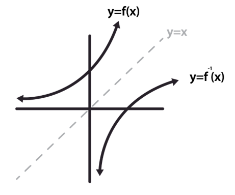
Inverse Functions
Inverse Function → in each output value is mapped from a unique input value
Ex. f(x): inputs on x-axis and outputs on y-axis (f(a) = b) →
f-1(x): inputs on y axis and outputs on x axis (f-1(b) = a)
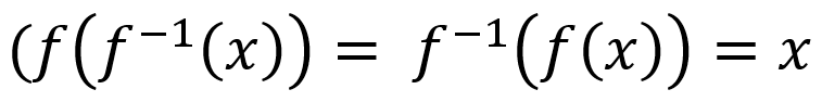
composite of function and inverse = identity function
 function’s domain and range → inverse function’s range and domain (respectively)
*domain may be restricted
Inverse of Exponential Functions
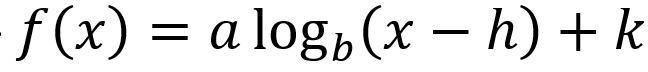
f(x) = a logb x with base b, where b > 0, b ≠ 1, and a ≠ 0
generally, exponential functions and log functions are inverse functions (reflections over h(x) = x)
└ f(x) = logb x and g(x) = bx → f (g(x)) = g( f(x)) = x
exponential growth → output values changing multiplicatively as input values change additively
logarithmic growth → output values changing additively as input values change multiplicative
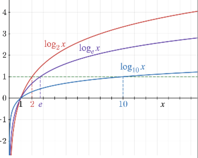
Logarithmic Functions
logbc = value b must be exponentially raised to in oder to obtain the value c
logbc if and only if ba = c (a & c = constants) (b > 0) (b ≠ 1)
if b not specified, log is common log with base 10 (b = 10)
used to model situations involving proportional growth or repeated multiplication
a logarithmic function can be constructed from a proportion and a real zero/ two input-output pairs
each unit represents a multiplicative change of the base of the log
domain of general form → any real number greater than 0
range of general form → all real numbers
If input values of the additive transformation function g(x) = f (x + k) are proportional over equal-length output value intervals à →(x) is logarithmic (Does not apply vice versa)
since inverse of exponential function → logarithmic functions are:
- always increasing or always decreasing
- always concave up or always concave down
- do not have extrema except on closed intervals
- do not have points of inflection
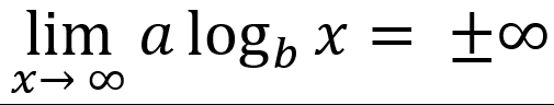
In general form, features of log function include:
-vertically asymptotic to x = 0
-end behavior is unbounded
└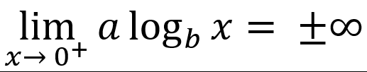 or
or
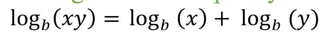
Log Product Property:
|
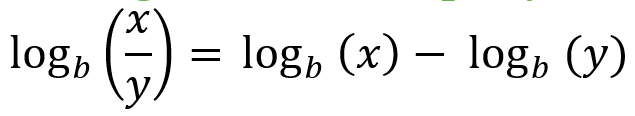
Log Quotient Property:
|
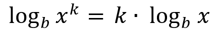
Log Exponential Property:
|
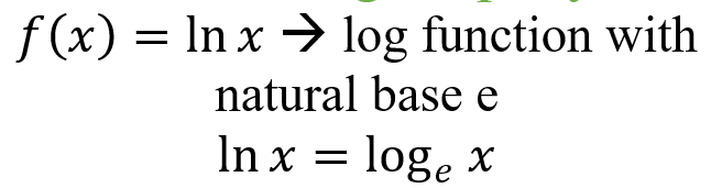
Natural Log Property:
|
Exponential and Logarithmic Equations and Inequalities
- must look for extraneous solutions
-exponential can be written as log functions
 combination of transformations of exponential function in general form *
 combination of transformation of log function in general form *
* inverse of function can be found by determining the inverse operation to reverse the mapping
Semi-Log Plots
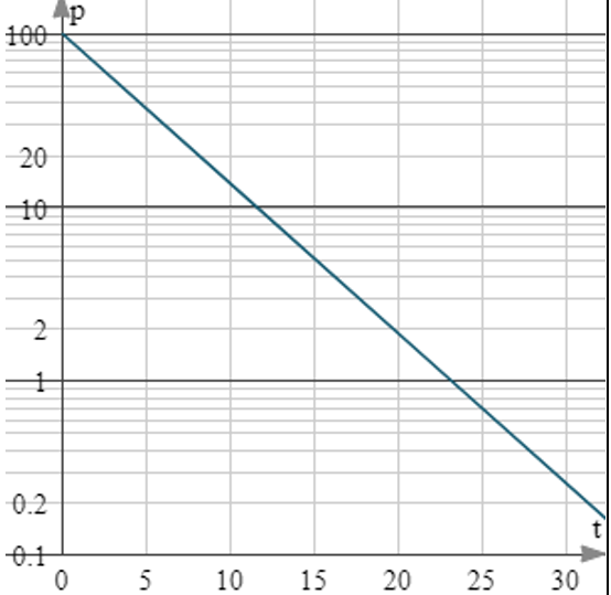
- y-axis is logarithmically scaled, while the x-axis is linearly scaled
- used to visualize exponential functions
- a constant does not need to be added to reveal that an exponential model is appropriate
- linear model for semi-log plot:
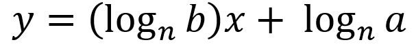 where n > 0 and n ≠ 0
└ linear rate of change: 
└ initial linear value:
Unit 3: Trigonometric and Polar Functions
3.1: Periodic Phenomena
Periodic Phenomena: occurrences or relationships that display a repetitive pattern over time or space.
Ex: undulating motion of waves, the circular rotation of clock hands, and the fluctuation in daylight hours throughout the year
Key Details of Graphs:
Periodic Function: A function that replicates a sequence of y-values at fixed intervals
Period: The gap between repetitions of a periodic function. Represents the length of one complete cycle
Intervals of Increase and Decrease: Define sets of x-values from the lower to the maximum point and from the upper to the minimum point, respectively
Concavity: when rate of intervals of increase/decrease is changing
Average Rate of Change: change in output divided by the change in input
3.2: Sine, Cosine, and Tangent
Standard Position Angles
Angles are like shapes formed where two lines, parts, or beams meet.
When describing an angle by its rotation, the starting point is called the initial side, and the endpoint after the rotation is the terminal side. This is called standard position
Rotations include positive and negative angles
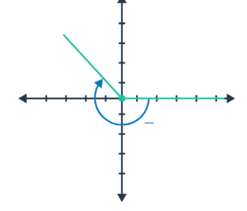
Standard Position: If an angle's initial side is parallel to the positive x-axis and its vertex is at the origin, it is said to be in the standard position.
Initial Side: The ray on the x-axis
Terminal Side: An angle's other ray in standard position
Positive Angle: When something is rotated counterclockwise
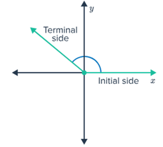
Negative Angle: When something is rotated clockwise
Radian Angle Measures
Can find the measure of an angle in radians by using the formula θ=s/r, where s is the arc length, and r is the circle's radius.
With circles with a radius of one unit, an angle of 11 radians would be the measure of an angle subtended by an arc of length 11 units.
The entire distance around a circle with a radius of one unit, or its circumference C, is 2π (since C=2πr). This means a complete turn around the circle corresponds to an angle of 2π radians, equivalent to 6.28 radians or 360 degrees.
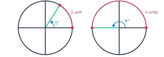
Since half a circle is π radians (as π radians equals 180 degrees), angles can be expressed as radians as fractions of π.
1 | 3/4 | 2/3 | 1/2 | 1/3 | 1/4 | 1/6 | 1/8 | 1/12 | |
|---|---|---|---|---|---|---|---|---|---|
Measure in degrees | 360° | 270° | 240° | 180° | 120° | 90° | 60° | 45° | 30° |
Measure in radians | 2π | 3/2π | 4/3π | π | 2/3π | π/2 | π/3 | π/4 | π/6 |
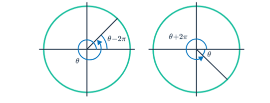
Coterminal Angles
Angles spin more than once, and their measures go beyond 2π radians.
Due to how angles are defined through rotation, it's conceivable to have two angles sharing the same starting and ending positions but having different measures. These related angles are known as coterminal angles.

If two angles end up in the same position, one might be a full rotation or more ahead or behind the other. The difference in their measures is like going around the circle several times.
For the unit circle (a circle with a radius of one), angles measured starting from the positive x-axis. Even if an angle goes beyond one complete turn around the circle, its trigonometric functions are related to those of an angle in the first quadrant.
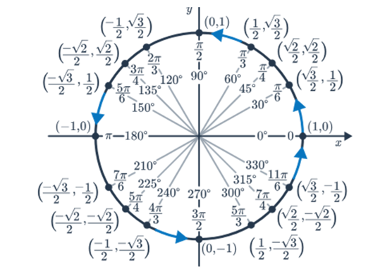
3.3: Sine and Cosine Functions Values
Sine and Cosine Functions and the Unit Circle
Special Triangles:
Special triangles on the unit circle aid in evaluating trigonometric functions with exact ratios.
45°-45°-90° Triangle:
Side lengths ratio - 1:1:1 times square root of 2
30°-60°-90° Triangle:
Side lengths ratio -1: 1 times square root of 3: 2
To Calculate:
Calculate the legs of each triangle, keeping your answer in fraction form.
Write the ordered pair that represents the endpoint of each radius on each unit circle.
3.4: Sine and Cosine Functions Values
Graphing the Sine Function
Use unit circle angles for x-axis representation.
Coordinate range: [−1,1] for the y-axis.
Explore the relationship between the unit circle and the sine graph.
Graphing the Cosine Function
Use unit circle angles for x-axis representation.
Coordinate range: [−1,1] for the x-axis.
Explore the relationship between the unit circle and the cosine graph.
3.5: Sinusoidal Functions
Sinusoidal Functions
Sine (sinθ) and cosine (cosθ) functions share a sinusoidal nature, exhibiting the same shape and traits, elucidated through their phase shift.
Key Characteristics of the Sine Function
Phase Shift:
It denotes the horizontal shift in a sine or cosine function upon adding an angle.
For instance, π to sinθ results in sinθ+π.
The shift in direction becomes evident after isolating sinθ.
Example: If sinθ+π=0, then sinθ=−π.
Due to the negative measure of the added angle, sinθ shifts π units to the left.
Sine Function Transformation: sin(θ)→sin(θ+π)→cos(θ).
Key Characteristics of the Cosine Function
Phase Shift:
It represents the horizontal shift in sine or cosine functions upon adding an angle.
Analogous to the phase shift of the sine function.
Cosine Function Transformation: cos(θ)=sin(θ+π).
Features
Both sine and cosine functions possess sinusoidal traits, sharing the same shape and features.
The phase shift occurs with the addition of π.
Both are same
Sine function key features:
Domain: (−∞,∞)(−∞,∞)
Range: [−1,1][−1,1]
Period: 2π
Frequency: 1/2π
Amplitude: 1
Midline: y=0
Cosine function key features:
Domain: (−∞,∞)
Range: [−1,1]
Period: 2π
Frequency: 1/2π
Amplitude: 11
Midline: y=0
3.6: Sinusoidal Function Transformations
Transformations of Sine and Cosine Functions
Transformations modify the critical features of sine and cosine functions.
An exploration involving sliders helps understand the impact of changes on the graph.
Sinusoidal Function
Sinosoidal Function: A function in y=asin[b(x−c)]+d represents a sine wave pattern.
Parameters:
A (Amplitude): Vertical stretch for ∣a∣>1, vertical compression for ∣a∣<1, and reflection across the x-axis for a<0.
b (Period): 2π/b, with horizontal compression for ∣b∣>1, horizontal stretch for ∣b∣<1, and reflection across the y-axis for b<0.
c (Phase Shift): Horizontal translation by c units.
d (Vertical Shift): Vertical translation by d units.
3.7: Sinusoidal Function Context and Data Modeling
Interpreting, Verifying, and Reporting with Models
When dealing with periodic phenomena problems, select a suitable model and ensure its verification by applying it to a problem situation.
Reporting with a model involves presenting relevant information to the audience and providing enough detail for understanding without delving into technical algebraic work or confusing mathematical jargon.
3.8: The Tangent Function
Graphing the Tangent Function
The tangent function, f(θ)=tanθ, is periodic, with a domain and range based on the unit circle.
It's undefined where cosθ=0, leading to a discontinuous function with a period of π.
The tangent function, f(θ)=tanθ, is transformed by adjusting frequency and midline.
The general form of the tangent function is f(θ)=atan[b(θ−c)]+d.
Key Features
Tangent Function [tan(θ)]:
Domain: θ≠2π+nπ, n is any integer
Range: (−∞,∞)
x-Intercept: θ=nπ,n is any integer
y-Intercept: 0
Period: π
Amplitude: None
Midline: 0
Transformations of the Tangent Function
General Form: f(θ)=atan[b(θ−c)]+d
Vertical Stretch/Compression:
∣A∣>1 is a vertical stretch.
∣A∣<1 is a vertical compression.
A <0 is a reflection across the x-axis.
Period:
b>1 is a horizontal compression.
0<∣b∣<1 is a horizontal stretch.
b<0 is a reflection across the y-axis.
Phase Shift:
Horizontal translation by c units.
Vertical Translation:
Vertical translation by d units.
3.9: Inverse Trigonometric Function
Introduction to Inverse Trigonometric Functions
The inverse trigonometric functions: arcsin (sin-1), arccos (cos-1), and arctan (tan-1)
The reciprocal relationship holds f(f -1(x))=x and f -1(f(x))=x.
sin(arcsinx)=x and arcsin(sinx)=x
cos(arccosx)=x and arccos(cosx)=x
tan(arctan)=x and arctan(tanx)=x
Developing Analytical and Graphical Representations
Finding the inverse function involves reflecting the original function about the line y=x.
Crucially, the inverse function must be one-to-one and comprehensively cover the complete range of sine values.
Mathematicians often choose a domain, such as [−2π,2π], for sine, resulting in the representation sin-1(x).
This also applies to the functions of cosine and tangent
3.10: Trigonometric Equations and Inequalities
Solving Trigonometric Equations
Trigonometric equations involve one or more of the six trigonometric functions: sine, cosine, tangent, cosecant, secant, and cotangent
Addressing trigonometric equations requires various strategies, including inverse functions and algebraic manipulations.
Solve Using Reciprocal Functions
Reciprocal trigonometric functions, including cosecant (cscθ), secant (secθ), and cotangent (cotθ), relate to the fundamental trigonometric functions
cscθ=1/sinθ
secθ=1/cosθ
cotθ=cosθ/sinθ
Solve Using the Unit Circle
For any point (x,y) on the unit circle corresponding to an angle θ, the trigonometric functions are defined as follows:
x=cosθ
y=sinθ
x/y=tanθ
Utilizing the unit circle, solutions to equations like sinθ=0 are determined within specified domains.
3.11: Secant, Cosecant, and Cotangent Functions
Key Features and Characteristics
Cosecant Function:
Domain: θ≠nπ,n is any integer
Range: (−∞,−1]∪[1,∞)
x-Intercept: None
y-Intercept: None
Period: 2π
Amplitude: None
Midline: y=0
Secant Function:
Domain: θ≠(2n+1)π/2,n is any integer
Range: (−∞,−1]∪[1,∞)
x-Intercept: None
y-Intercept: y=1
Period: 2π
Amplitude: None
Midline: y=0
Cotangent Function:
Domain: θ≠nπ,n is any integer
Range: (−∞,∞)
x-Intercept: x=2π+nπ,n is any integer
y-Intercept: None
Period: π
Amplitude: None
Midline: y=0
3.12: Equivalent Representations of Trigonometric Functions
Pythagorean Identity
The Pythagorean identity relates the trigonometric functions of a right triangle.
sin2θ+cos2θ=1
Sine and Cosine Sum Identities:
sin(α+β)=sinαcosβ+cosαsinβ
cos(α+β)=cosαcosβ−sinαsinβ
These identities are valuable tools for rewriting expressions involving sums of angles.
3.13: Trigonometry and Polar Coordinates
Polar Coordinates
A polar coordinate system involves measurements of distance (r) from the origin and angle (θ) from the positive horizontal axis (polar axis).
Denoted as (r,θ), polar coordinates differ from Cartesian coordinates (x,y).
The rectangular plane is often called the Cartesian or rectangular coordinate system.
Convert complex numbers from rectangular (a+bi) to polar coordinates r(cosθ+isinθ), utilizing cosθ and sinθ to express x and y, respectively.
3.14: Polar Function Graphs
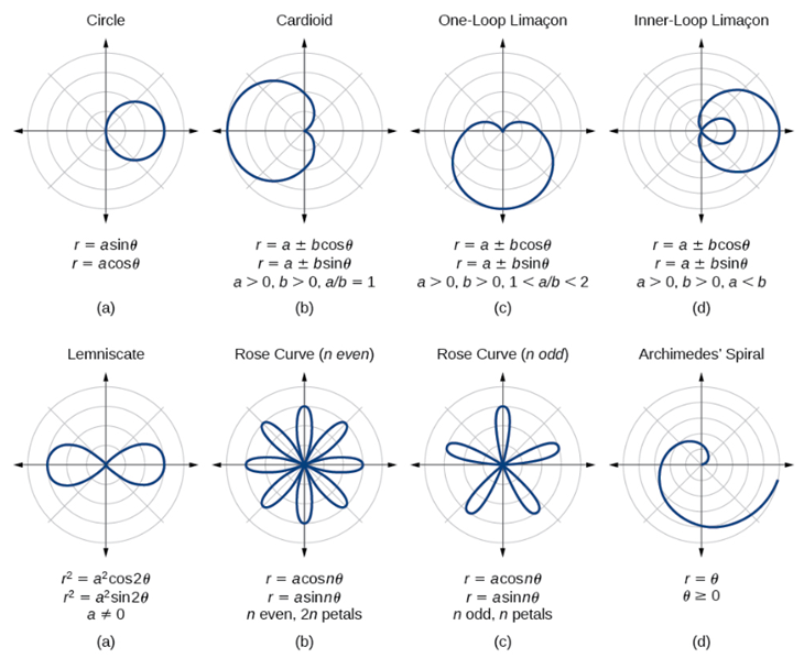
Circles
Polar functions express circles as r=a, where a is the radius.
General Form of a Circle: Circle equations in polar form: r=acosθ or r=asinθ.
Characteristics:
Positive a positions the circle right/above the origin; negative a positions it left/below.
Symmetry across the horizontal or vertical axis based on the sign.
Roses
Roses, represented as r=acos(kθ) or r=asin(kθ), have k determining the petal count.
Characteristics:
Odd k leads to k petals and even k results in 2k petals.
The angle between petals: 2π/k.
Symmetry across the horizontal or vertical axis.
Limacons
Limacons, given by r=a±bcosθ or r=a±bsinθ, have parameters a and b determining shape.
Shapes:
Dent (no loop) if ∣a∣>∣b∣.
Cardioid (heart shape) if ∣a∣=∣b∣.
Loop if ∣a∣<∣b∣.
Radius Characteristics:
Maximum radius:∣a∣+∣b∣.
Minimum radius: ∣a∣−∣b∣.
3.15: Rates of Change in Polar Functions
Characteristics of Polar Functions
Polar functions share similarities with other function types in analyzing characteristics like rate of change, increasing/decreasing intervals, positive/negative intervals, and extrema.
Polar Function Form: A polar function takes the form r=f(θ), where radii are output values and angles are input values.
Rate of Change: Positive, increasing, negative, and decreasing polar functions lead to an increasing distance from the origin (r).
Extrema: Transitions from increasing to decreasing or vice versa indicate relative extrema, representing points closest to or farthest from the origin.
Average Rate of Change: The average rate of change of r for θ over an interval is the ratio of the change in radius values to the change in θ. It signifies how the radius changes per radian.
Δr=(θ2)−f(θ1)/θ2−θ1f
Idea Summary
r positive: r positive, distance from origin increasing.
r negative: r negative, distance from origin decreasing.
r increasing: distance from origin increasing.
r decreasing: distance from origin decreasing.
Average rate of change formula: Δr/Δθ=f(θ2)−f(θ1)/θ2−θ1
Unit 4: Functions Involving Parameters, Vectors, and Matrices
4.1 Parametric Functions
Understanding Parametric Functions:
Parametric functions introduce the concept of coordinates (xi,yi) at specific times ti, expressed as functions of t. A parametric function, f(t)=(x(t),y(t)), encapsulates two functions, x and y, dependent on the parameter t. For instance, consider f(t)=(t2,2t) where x(t)=t2 and y(t)=2t.
Parametric functions encompass two dependent variables, x and y, reliant on a single independent variable, t. The parameter t influences the values of x and y.
Graphing and Tabulating Parametric Functions:
Visualizing parametric functions involves creating a graph by plotting points from a table of values. This representation enhances the understanding of the function's properties, aiding in analysis and interpretation.
4.2 Parametric Functions Modeling Planar Motion
Analyzing Particle Motion:
A detailed examination of the individual parametric equations x(t) and y(t) is necessary to scrutinize the motion. These equations elucidate the horizontal and vertical components of the particle's motion, respectively. The graphical representation of a parametric function illustrates the particle's path in the plane over time, with each point on the graph corresponding to a specific position of the particle at a given time.
Horizontal and Vertical Extrema:
Horizontal extrema denotes the furthest points in the horizontal direction, determined by the maximum and minimum values of x(t). Similarly, vertical extrema represents the furthest points in the vertical direction, identified by the maximum and minimum values of y(t). Recognizing these extrema augments the comprehension of the particle's trajectory.
4.3 Parametric Functions and Rates of Change
Direction and Rate of Change:
Parametric planar motion functions serve as models defining a particle's position in a plane concerning a parameter, typically time t. Analyzing the direction involves scrutinizing the independent components x and y separately. As the parameter t increases, the direction of motion is deciphered by assessing the functions x(t) and y(t).
Average Rate of Change:
The average rate of change in parametric functions is a pivotal concept providing insights into a particle's motion in the plane. By computing the average rate of change for x(t) and y(t) independently, valuable information about horizontal and vertical changes in the particle's position over time is obtained.
Direction of Motion:
Determining the direction of motion entails evaluating whether x(t) o y(t) is increasing or decreasing as t progresses. This analysis is crucial for understanding the orientation of a particle's movement in the plane.
Unit Circle and Special Angles:
The unit circle, with special angles labeled, aids in visualizing angles and directions. These special angles guide the analysis of motion and provide a reference for understanding the intricacies of parametric functions.
4.4 Parametrically Defined Functions
Modeling Motion Around a Circle:
A unit circle, centered at a Cartesian plane's origin (0,0), becomes a focal point. Each point on the circle can be represented by coordinates (cosθ, sinθ), where θ is the angle formed by the positive x-axis and a line segment from the origin to the point. Transformations, including scaling, translating, and reflecting, allow adjustments to basic parametric equations for circular motion.
Parametrizing a Linear Path:
Parametric equations transcend circular applications and prove invaluable for describing linear motion.
Example: A car moving from point A to point B. The initial and final positions and the constant speed denoted by parameter t formulate parametric equations that represent the car's linear motion.
4.5 Implicitly Defined Functions
Graphs of Implicitly Defined Functions:
Implicitly defined functions, a unique breed of equations involving two variables, operate without explicitly expressing the dependent variable in terms of the independent variable. Unlike explicit functions, implicit functions can represent one or more functions within a single equation, unbounded by the constraints of direct expression.
Variation in Implicitly Defined Functions:
Implicitly defined functions describe complex relationships between variables within a single equation. The resulting graph can take diverse forms, including a single curve, multiple disjoint curves, or even an infinite number of curves. To graph an implicitly defined function, solutions to the equation are sought, unveiling points on the graph where the relationship between variables holds true.
4.6 Conic Sectors
Expressing a Curve Parametrically
In the mathematical realm, curves present themselves in diverse ways. Two common approaches are explicit representation (where y depends on x) and the more adaptable parametric representation.
Basics of Parametric Expression
Parametric representation involves defining x and y as functions of an additional variable t. As t varies, x and y evolve, outlining the curve. The resultant x(t) and y(t) functions are the parametric equations of the curve.
Validating this representation entails substituting x(t) and y(t) back into the original equation. If the equation holds for all t values in its domain, the parametric representation is accurate.
Special Cases: Function and Its Inverse
For a function f of x, parametrizing y=f(x) involves expressing both x and y as functions of t, generating (x(t),y(t))=(t,f(t)). If f has an inverse, the inverse can be parametrized as (x(t),y(t))=(f(t),t).
Parametric Formulas for Conic Sections
In examining conic sections (parabolas, ellipses, and hyperbolas), particular formulas facilitate parametric representation, framing x and y in terms of t.
Parabolas
Parametrizing a parabola involves solving for either x or y. The resulting parametric equations are (x(t),y(t))=(t,f(t)) or (x(t),y(t))=(f(t),t), determined by the chosen variable for parametrization.
Ellipses
Ellipses, closed curves defined by distances from two foci, use trigonometric functions for parametrization. The parametric equations feature cos and sin functions, articulating x and y in relation to t.
Hyperbolas
Parametrizing hyperbolas, where the difference of distances to two fixed points is constant, involves utilizing secant and tangent functions. Depending on orientation, hyperbolas open left/right or up/down, with parametric equations embracing these trigonometric functions.
4.8 Vectors
Characteristics of Vectors
Defining Vectors: Vectors, illustrated as directed line segments, encapsulate both direction and magnitude. Their significance permeates disciplines like physics and engineering, where quantities possess directional and size attributes.
Components and Parts: In the two-dimensional plane, vectors can be decomposed into components. Each part, representing a dimension, is termed a component.
Representation in the Plane
Geometric Representation: Placing a vector in the plane involves defining its tail and head, symbolizing the beginning and end of the line segment, respectively.
Two-Dimensional Influence: Vectors in two dimensions exert influence in two distinct directions, envisioning a dualistic impact.
Vector Components
Component Identification: A vector with components a and b is often represented as (a,b) or ⟨a,b⟩. The process involves calculating differences along each dimension.
Magnitude and Direction
Vector Analysis: Considering a vector ⟨a,b⟩, its magnitude is determined by the Pythagorean theorem: ⟨a,b⟩∣=a2+b2.
Direction Determination: The direction aligns with the line segment from the origin to the point ⟨a,b⟩, and trigonometry aids in extracting components.
Vector Operations
Scalar Multiplication: When a vector ⟨a,b⟩ is multiplied by a scalar k, the result ⟨ka,kb⟩ is parallel to the original vector.
Vector Addition: The sum of vectors ⟨a1,b1⟩ and ⟨a2,b2⟩ is ⟨a1+a2,b1+b2⟩. Addition involves combining corresponding components.
Dot Product: The dot product of vectors ⟨a1,b1⟩ and ⟨a2,b2⟩ is a1a2+b1b2. It also correlates with magnitudes and angles.
Unit Vectors: Unit vectors with a magnitude of 11 represent direction. Normalizing vectors involves dividing by their magnitude.
Measures and Analysis
Angle Computation: The angle θ between vectors ⟨a1,b1⟩ and ⟨a2,b2⟩ is determined using the arccosine function.
Law of Cosines: cos(θ)=∣u∣⋅∣v∣⟨u⟩⋅⟨v⟩, for angles between vectors.
Law of Sines: sin(α)=∣w∣∣u∣=sin(β)=∣w∣∣v∣=sin(γ), for side lengths and angles in vector-formed triangles.
4.9 Vector-Valued Functions
Position Vectors
Position vectors are crucial for understanding plane or space movement.
They describe a particle's position using a vector originating from the origin and ending at the particle's location.
Vector-Valued Function:
Expresses particle position in a plane using a vector-valued function:
p(t)=ix(t)+jy(t) or p(t)=⟨x(t),y(t)⟩.
Here, x(t) and y(t) are parametric functions representing particle coordinates at time t.
The magnitude of p(t) provides the particle's distance from the origin.
Example: If x(t)=2t+1 and y(t)=3t−2, the position vector is p(t)=(2t+1)i+(3t−2)j.
Velocity Vectors
Vector-Valued Function:
The velocity of a particle in a plane is expressed by v(t)=⟨x(t),y(t)⟩.
Direction indicates motion direction (right/left, up/down).
Magnitude gives particle speed at a specific time.
The Magnitude of Velocity:
Calculated by the square root of the sum of squared x and y components.
4.10 Matrices
Matrix Dimensions
Matric Dimension: A matrix is an ordered array with n rows and m columns, denoted as n×m.
Classification by Order:
Square Matrix: n×n
Example: 3×3 matrix
[123]
[456]
[789]
Row Matrix: 1×n
Example:1×3 matrix
[1,2,3]
Column Matrix: n×1
Example: 3×1 matrix
[1]
[4]
[7]
Matrix Elements: Denoted by amn, representing the element in the m-th row and n-th column.
Matrix Multiplication
Matrix Equality: Matrices are equal if they have the same order and each corresponding element is equal.
Matrix Multiplication: Matrices can be multiplied if the number of columns in the first matrix equals the number of rows in the second matrix.
Resulting matrix dimensions: m×n, where m is the number of rows of the first matrix and n is the number of columns of the second matrix.
Not commutative: A⋅B≠B⋅A.
Multiplication Process: Each element in the resulting matrix is the dot product of the corresponding row from the first matrix and column from the second matrix.
4.11 The Inverse and Determinant of a Matrix
Identity Matrix and Determinants
Identity Matrix (I): Special square matrix with 1's on the main diagonal and 0's elsewhere; Denoted as I.
Matrix Multiplication with Identity Matrix: When a square matrix is multiplied by its corresponding identity matrix, the original matrix results.
Determinant:
Scalar value with applications in invertibility and vector areas.
For a 2×2 matrix A=[ab, cd], the determinant is calculated as det(A)=ad−bc.
Area of Parallelogram and Determinant
Parallelogram Formed by Vectors: If det(A)≠0, vectors formed by the column and row vectors are not parallel.
Area of Parallelogram: The absolute value of the determinant represents the area of the parallelogram formed by vectors.
The Inverse of a 2×2 Matrix
Inverse Existence: A square matrix A has an inverse (A−1) if and only if det(A)≠0.
Inverse Formula: For a 2×2 matrix A=[ab, cd], the inverse is given by A1=1/det(A)[d −b,−c a].
4.12 Linear Transformations and Matrices
Understanding Linear Transformations
Linear Transformations: A linear transformation is a function that maps input vectors to output vectors while preserving vector addition and scalar multiplication operations.
A linear transformation L from a vector space R2 to another vector space R2 is expressed as L(u+v)=L(u)+L(v) and L(cv)=cL(v).
Linear transformations preserve vector addition and scalar multiplication.
Zero Vector Mapping: Linear transformations map the zero vector to the zero vector: (0)=0L(0)=0.
Vectors and Matrices Representation
Vectors in 2R2 can be represented using matrices.
A single vector is expressed as a 2×1 matrix, and a set of n vectors is represented as a 2×n matrix.
Example: If v=[xy], it is represented as a 2×1 matrix: v=[xy].
Linear Transformations and Matrices
Transformation Matrix (2x2): For a linear transformation L from R2 to R2, there exists a unique 2×2 matrix A such that L(v)=Av for all vectors in R2
Matrix to Linear Transformation (2x2): Conversely, for a given 2×2 matrix A, the function L(v)=Av is a linear transformation.
Output Vector Calculation:
To find the output vectors for a linear transformation L(v)=Av, multiply the 2×2 transformation matrix A with the 2×n matrix of input vectors, resulting in a 2×n matrix of output vectors.
4.13 Matrices as Functions
Linear Transformation and Matrices
General Form of A Linear Transformation: Represented by the matrix [a11 a12, a21 a22].
Matrix Elements Correspondence: Each element in the matrix corresponds to a coefficient in the transformation, and when the matrix multiplies a vector, it produces the same result as the linear transformation.
Unit Vector Mapping: Mapping unit vectors (e.g., i=⟨1,0⟩, j=⟨0,1⟩) under a linear transformation helps determine the associated matrix.
Special Matrices: Special matrices correspond to specific transformations (e.g., rotation matrix for counterclockwise rotation by θ degrees).
Determinant Significance: Its absolute value gives the scale factor under the transformation.
Composition of Two Linear Transformations
Linear Transformation Composition: Where one transformation is applied followed by another. The composition of two linear transformations is itself a linear transformation.
Composition Matrix Rule: The matrix associated with the composition is the product of the matrices associated with each transformation.
Matrix Multiplication Order: Matrix multiplication is not commutative; the order of transformations matters
Inverse of a Linear Transformation
Linear Transformation Inverse: Undoes the effect of the original one. It is represented by the inverse of the matrix for the original transformation.
Inverse Matrix Conditions: Only square matrices with a nonzero determinant can potentially have an inverse.
Inverse Matrix Calculation: The inverse of a 2×2 matrix [a c,b d] is given by 1/ad−bc [d−c−ba] if ad−bc ≠ 0.
4.14 Matrices Modeling Contexts
Matrices as Dynamic Models
Analyzing Transitions:
Employing matrices proves to be an adept strategy for modeling transitions between diverse states, offering a versatile framework applicable across various scenarios.
Defining State Changes:
Transitions embody shifts from one state to another, encapsulating alterations within a system over discrete temporal intervals.
Quantifying Changes:
Quantification of these transitions typically involves rates expressed as percentage changes, reflecting the dynamism inherent in the system.
Transition Matrix Essence:
At the heart of this modeling lies the transition matrix, a square matrix, often 2×2, encoding the rates of transition between different states.