


AP Precalculus Unit 4 Notes
4.1 Parametric Functions
Understanding Parametric Functions:
Parametric functions introduce the concept of coordinates (xi,yi) at specific times ti, expressed as functions of t. A parametric function, f(t)=(x(t),y(t)), encapsulates two functions, x and y, dependent on the parameter t. For instance, consider f(t)=(t2,2t) where x(t)=t2 and y(t)=2t.
Parametric functions encompass two dependent variables, x and y, reliant on a single independent variable, t. The parameter t influences the values of x and y.
Graphing and Tabulating Parametric Functions:
Visualizing parametric functions involves creating a graph by plotting points from a table of values. This representation enhances the understanding of the function's properties, aiding in analysis and interpretation.
4.2 Parametric Functions Modeling Planar Motion
Analyzing Particle Motion:
A detailed examination of the individual parametric equations x(t) and y(t) is necessary to scrutinize the motion. These equations elucidate the horizontal and vertical components of the particle's motion, respectively. The graphical representation of a parametric function illustrates the particle's path in the plane over time, with each point on the graph corresponding to a specific position of the particle at a given time.
Horizontal and Vertical Extrema:
Horizontal extrema denotes the furthest points in the horizontal direction, determined by the maximum and minimum values of x(t). Similarly, vertical extrema represents the furthest points in the vertical direction, identified by the maximum and minimum values of y(t). Recognizing these extrema augments the comprehension of the particle's trajectory.
4.3 Parametric Functions and Rates of Change
Direction and Rate of Change:
Parametric planar motion functions serve as models defining a particle's position in a plane concerning a parameter, typically time t. Analyzing the direction involves scrutinizing the independent components x and y separately. As the parameter t increases, the direction of motion is deciphered by assessing the functions x(t) and y(t).
Average Rate of Change:
The average rate of change in parametric functions is a pivotal concept providing insights into a particle's motion in the plane. By computing the average rate of change for x(t) and y(t) independently, valuable information about horizontal and vertical changes in the particle's position over time is obtained.
Direction of Motion:
Determining the direction of motion entails evaluating whether x(t) o y(t) is increasing or decreasing as t progresses. This analysis is crucial for understanding the orientation of a particle's movement in the plane.
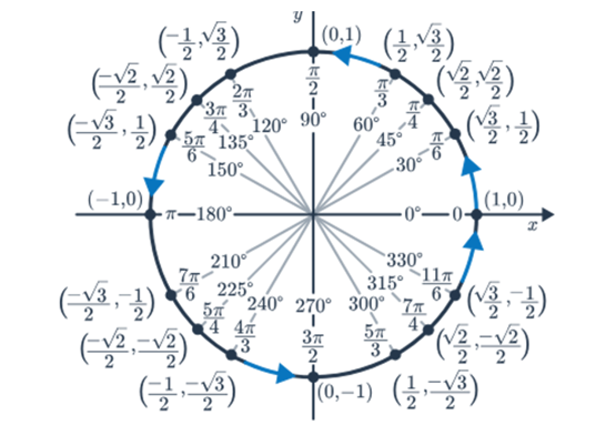
Unit Circle and Special Angles:
The unit circle, with special angles labeled, aids in visualizing angles and directions. These special angles guide the analysis of motion and provide a reference for understanding the intricacies of parametric functions.
4.4 Parametrically Defined Functions
Modeling Motion Around a Circle:
A unit circle, centered at a Cartesian plane's origin (0,0), becomes a focal point. Each point on the circle can be represented by coordinates (cosθ, sinθ), where θ is the angle formed by the positive x-axis and a line segment from the origin to the point. Transformations, including scaling, translating, and reflecting, allow adjustments to basic parametric equations for circular motion.
Parametrizing a Linear Path:
Parametric equations transcend circular applications and prove invaluable for describing linear motion.
o Example: A car moving from point A to point B. The initial and final positions and the constant speed denoted by parameter t formulate parametric equations that represent the car's linear motion.
4.5 Implicitly Defined Functions
Graphs of Implicitly Defined Functions:
Implicitly defined functions, a unique breed of equations involving two variables, operate without explicitly expressing the dependent variable in terms of the independent variable. Unlike explicit functions, implicit functions can represent one or more functions within a single equation, unbounded by the constraints of direct expression.
Variation in Implicitly Defined Functions:
Implicitly defined functions describe complex relationships between variables within a single equation. The resulting graph can take diverse forms, including a single curve, multiple disjoint curves, or even an infinite number of curves. To graph an implicitly defined function, solutions to the equation are sought, unveiling points on the graph where the relationship between variables holds true.
4.6 Conic Sectors
Expressing a Curve Parametrically
In the mathematical realm, curves present themselves in diverse ways. Two common approaches are explicit representation (where y depends on x) and the more adaptable parametric representation.
Basics of Parametric Expression
Parametric representation involves defining x and y as functions of an additional variable t. As t varies, x and y evolve, outlining the curve. The resultant x(t) and y(t) functions are the parametric equations of the curve.
Validating this representation entails substituting x(t) and y(t) back into the original equation. If the equation holds for all t values in its domain, the parametric representation is accurate.
Special Cases: Function and Its Inverse
For a function f of x, parametrizing y=f(x) involves expressing both x and y as functions of t, generating (x(t),y(t))=(t,f(t)). If f has an inverse, the inverse can be parametrized as (x(t),y(t))=(f(t),t).
Parametric Formulas for Conic Sections
In examining conic sections (parabolas, ellipses, and hyperbolas), particular formulas facilitate parametric representation, framing x and y in terms of t.
Parabolas
Parametrizing a parabola involves solving for either x or y. The resulting parametric equations are (x(t),y(t))=(t,f(t)) or (x(t),y(t))=(f(t),t), determined by the chosen variable for parametrization.
Ellipses
Ellipses, closed curves defined by distances from two foci, use trigonometric functions for parametrization. The parametric equations feature cos and sin functions, articulating x and y in relation to t.
Hyperbolas
Parametrizing hyperbolas, where the difference of distances to two fixed points is constant, involves utilizing secant and tangent functions. Depending on orientation, hyperbolas open left/right or up/down, with parametric equations embracing these trigonometric functions.
4.8 Vectors
Characteristics of Vectors
Defining Vectors: Vectors, illustrated as directed line segments, encapsulate both direction and magnitude. Their significance permeates disciplines like physics and engineering, where quantities possess directional and size attributes.
Components and Parts: In the two-dimensional plane, vectors can be decomposed into components. Each part, representing a dimension, is termed a component.
Representation in the Plane
Geometric Representation: Placing a vector in the plane involves defining its tail and head, symbolizing the beginning and end of the line segment, respectively.
Two-Dimensional Influence: Vectors in two dimensions exert influence in two distinct directions, envisioning a dualistic impact.
Vector Components
Component Identification: A vector with components a and b is often represented as (a,b) or ⟨a,b⟩. The process involves calculating differences along each dimension.
Magnitude and Direction
Vector Analysis: Considering a vector ⟨a,b⟩, its magnitude is determined by the Pythagorean theorem: ⟨a,b⟩∣=a2+b2.
Direction Determination: The direction aligns with the line segment from the origin to the point ⟨a,b⟩, and trigonometry aids in extracting components.
Vector Operations
Scalar Multiplication: When a vector ⟨a,b⟩ is multiplied by a scalar k, the result ⟨ka,kb⟩ is parallel to the original vector.
Vector Addition: The sum of vectors ⟨a1,b1⟩ and ⟨a2,b2⟩ is ⟨a1+a2,b1+b2⟩. Addition involves combining corresponding components.
Dot Product: The dot product of vectors ⟨a1,b1⟩ and ⟨a2,b2⟩ is a1a2+b1b2. It also correlates with magnitudes and angles.
Unit Vectors: Unit vectors with a magnitude of 11 represent direction. Normalizing vectors involves dividing by their magnitude.
Measures and Analysis
Angle Computation: The angle θ between vectors ⟨a1,b1⟩ and ⟨a2,b2⟩ is determined using the arccosine function.
Law of Cosines: cos(θ)=∣u∣⋅∣v∣⟨u⟩⋅⟨v⟩, for angles between vectors.
Law of Sines: sin(α)=∣w∣∣u∣=sin(β)=∣w∣∣v∣=sin(γ), for side lengths and angles in vector-formed triangles.
4.9 Vector-Valued Functions
Position Vectors
Position vectors are crucial for understanding plane or space movement.
They describe a particle's position using a vector originating from the origin and ending at the particle's location.
Vector-Valued Function:
Expresses particle position in a plane using a vector-valued function:
p(t)=ix(t)+jy(t) or p(t)=⟨x(t),y(t)⟩.
Here, x(t) and y(t) are parametric functions representing particle coordinates at time t.
The magnitude of p(t) provides the particle's distance from the origin.
Example: If x(t)=2t+1 and y(t)=3t−2, the position vector is p(t)=(2t+1)i+(3t−2)j.
Velocity Vectors
Vector-Valued Function:
The velocity of a particle in a plane is expressed by v(t)=⟨x(t),y(t)⟩.
Direction indicates motion direction (right/left, up/down).
Magnitude gives particle speed at a specific time.
The Magnitude of Velocity:
Calculated by the square root of the sum of squared x and y components.
4.10 Matrices
Matrix Dimensions
Matric Dimension: A matrix is an ordered array with n rows and m columns, denoted as n×m.
Classification by Order:
Square Matrix: n×n
Example: 3×3 matrix
[123]
[456]
[789]
Row Matrix: 1×n
Example:1×3 matrix
[1,2,3]
Column Matrix: n×1
Example: 3×1 matrix
[1]
[4]
[7]
Matrix Elements: Denoted by amn, representing the element in the m-th row and n-th column.
Matrix Multiplication
Matrix Equality: Matrices are equal if they have the same order and each corresponding element is equal.
Matrix Multiplication: Matrices can be multiplied if the number of columns in the first matrix equals the number of rows in the second matrix.
Resulting matrix dimensions: m×n, where m is the number of rows of the first matrix and n is the number of columns of the second matrix.
Not commutative: A⋅B≠B⋅A.
Multiplication Process: Each element in the resulting matrix is the dot product of the corresponding row from the first matrix and column from the second matrix.
4.11 The Inverse and Determinant of a Matrix
Identity Matrix and Determinants
Identity Matrix (I): Special square matrix with 1's on the main diagonal and 0's elsewhere; Denoted as I.
Matrix Multiplication with Identity Matrix: When a square matrix is multiplied by its corresponding identity matrix, the original matrix results.
Determinant:
Scalar value with applications in invertibility and vector areas.
For a 2×2 matrix A=[ab, cd], the determinant is calculated as det(A)=ad−bc.
Area of Parallelogram and Determinant
Parallelogram Formed by Vectors: If det(A)≠0, vectors formed by the column and row vectors are not parallel.
Area of Parallelogram: The absolute value of the determinant represents the area of the parallelogram formed by vectors.
The Inverse of a 2×2 Matrix
Inverse Existence: A square matrix A has an inverse (A−1) if and only if det(A)≠0.
Inverse Formula: For a 2×2 matrix A=[ab, cd], the inverse is given by A1=1/det(A)[d −b,−c a].
4.12 Linear Transformations and Matrices
Understanding Linear Transformations
Linear Transformations: A linear transformation is a function that maps input vectors to output vectors while preserving vector addition and scalar multiplication operations.
A linear transformation L from a vector space R2 to another vector space R2 is expressed as L(u+v)=L(u)+L(v) and L(cv)=cL(v).
Linear transformations preserve vector addition and scalar multiplication.
Zero Vector Mapping: Linear transformations map the zero vector to the zero vector: (0)=0L(0)=0.
Vectors and Matrices Representation
Vectors in 2R2 can be represented using matrices.
A single vector is expressed as a 2×1 matrix, and a set of n vectors is represented as a 2×n matrix.
Example: If v=[xy], it is represented as a 2×1 matrix: v=[xy].
Linear Transformations and Matrices
Transformation Matrix (2x2): For a linear transformation L from R2 to R2, there exists a unique 2×2 matrix A such that L(v)=Av for all vectors in R2
Matrix to Linear Transformation (2x2): Conversely, for a given 2×2 matrix A, the function L(v)=Av is a linear transformation.
Output Vector Calculation:
To find the output vectors for a linear transformation L(v)=Av, multiply the 2×2 transformation matrix A with the 2×n matrix of input vectors, resulting in a 2×n matrix of output vectors.
4.13 Matrices as Functions
Linear Transformation and Matrices
General Form of A Linear Transformation: Represented by the matrix [a11 a12, a21 a22].
Matrix Elements Correspondence: Each element in the matrix corresponds to a coefficient in the transformation, and when the matrix multiplies a vector, it produces the same result as the linear transformation.
Unit Vector Mapping: Mapping unit vectors (e.g., i=⟨1,0⟩, j=⟨0,1⟩) under a linear transformation helps determine the associated matrix.
Special Matrices: Special matrices correspond to specific transformations (e.g., rotation matrix for counterclockwise rotation by θ degrees).
Determinant Significance: Its absolute value gives the scale factor under the transformation.
Composition of Two Linear Transformations
Linear Transformation Composition: Where one transformation is applied followed by another. The composition of two linear transformations is itself a linear transformation.
Composition Matrix Rule: The matrix associated with the composition is the product of the matrices associated with each transformation.
Matrix Multiplication Order: Matrix multiplication is not commutative; the order of transformations matters
Inverse of a Linear Transformation
Linear Transformation Inverse: Undoes the effect of the original one. It is represented by the inverse of the matrix for the original transformation.
Inverse Matrix Conditions: Only square matrices with a nonzero determinant can potentially have an inverse.
Inverse Matrix Calculation: The inverse of a 2×2 matrix [a c,b d] is given by 1/ad−bc [d−c−ba] if ad−bc ≠ 0.
4.14 Matrices Modeling Contexts
Matrices as Dynamic Models
Analyzing Transitions:
Employing matrices proves to be an adept strategy for modeling transitions between diverse states, offering a versatile framework applicable across various scenarios.
Defining State Changes:
Transitions embody shifts from one state to another, encapsulating alterations within a system over discrete temporal intervals.
Quantifying Changes:
Quantification of these transitions typically involves rates expressed as percentage changes, reflecting the dynamism inherent in the system.
Transition Matrix Essence:
At the heart of this modeling lies the transition matrix, a square matrix, often 2×2, encoding the rates of transition between different states.