
Chapters 24.3-24.5: Basic Macroeconomic Models
The Interest-Rate–Investment Relationship
The investment decision is a marginal-benefit–marginal-cost decision
The marginal benefit from investment is the expected rate of return businesses hope to realize. The marginal cost is the interest rate that must be paid for borrowed funds.
Expected rate of return (r)
Expected rate of return::
The increase in profit a firm anticipates it will obtain by purchasing capital or engaging in research and development (R&D); expressed as a percentage of the total cost of the investment (or R&D) activity.
Expected profit = net expected revenue - cost of investment
Expected rate of return (r) = expected profit / cost of investment
This is an expected rate of return, not a guaranteed rate of return
Real interest rate (i)
real interest rate = nominal interest rate - inflation premium
firms will not invest if the real interest rate (i) exceeds the expected rate of return (r)
firms will invest to the point where r = i because then it will have undertaken all investments for which r is greater than i.
This guideline applies even if a firm finances the investment internally out of funds saved from past profit rather than borrowing the funds
real rate of interest (without inflation premium), rather than the nominal rate, is crucial in making investment decisions.
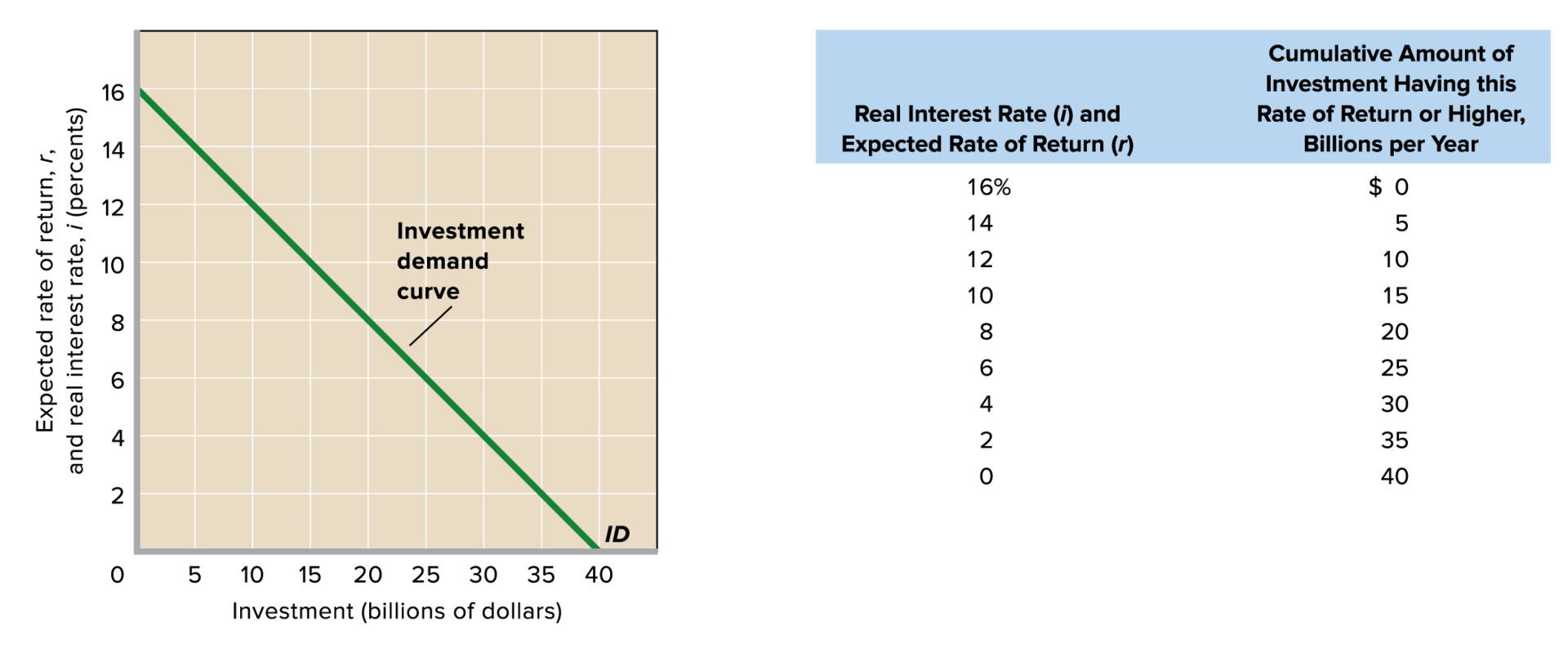
Investment demand curve
we now move from a single firm’s investment decision to total demand for investment goods by the entire business sector.
To cumulate the investment demanded for each rate of return, r, we add the amounts of investment that will yield each particular rate of return r or higher.
ex. at a real interest rate of 10%, $15 billion dollars of investment goods will be demanded
Because of the marginal-benefit–marginal-cost rule that investment projects should be undertaken up to the point where r = i, the real interest rate and expected rate of return are both added to the vertical axis
There is an inverse relationship because the higher the interest rate (“cost of investment”), the less firms will want to invest
Shifts of the Investment Demand Curve
changes in real interest rates cause movements along the invest-demand curve
The non-interest rate determinants of investment demand cause shifts of the entire curve
Generally, these are factors that make businesses collectively expect higher or lower rates of return on their investments
A higher expected rate of return shifts the curve to the right
A lower expected rate of return shifts the curve to the left
6 Non-interest rate determinants of investment demand
Acquisition, maintenance, and operating costs
When these costs rise, the expected rate of return from prospective investment projects falls and the investment demand curve shifts to the left. Lower costs, in contrast, shift it to the right.
Business taxes
Firms look to expected returns after taxes in making their investment decisions
An increase in business taxes lowers the expected profitability of investments and shifts the investment demand curve to the left; a reduction of business taxes shifts it to the right.
Technological change
Technological progress—the development of new products, improvements in existing products, and the creation of new machinery and production processes—stimulates investment and increases expected rate of return, shifting the investment demand curve to the right.
Stock of capital goods on hand
When the economy is overstocked with production facilities and firms have excessive inventories of finished goods, the expected rate of return on new investment declines.
Firms with excess production capacity have little incentive to invest in new capital. Therefore, the investment demand curve shifts leftward.
When the economy is understocked with production facilities and when firms are selling their output as fast as they can produce it, the expected rate of return on new investment increases and the investment demand curve shifts rightward.
Planned inventory changes
Investment-demand curve isn’t affected by unplanned inventory changes
If firms are planning to increase their inventories (ex. because of higher expected sales), the investment demand curve shifts to the right.
If firms are planning on decreasing their inventories (ex. because of lower expected sales), the investment demand curve shifts to the left.
Expectations
Expectations are based on forecasts of future business conditions as well as elusive factors like changes in the domestic political climate, international relations, population growth, and consumer tastes.
If executives become more optimistic about future sales, costs, and profits, the investment demand curve will shift to the right; a pessimistic outlook will shift the curve to the left.
Instability of investment
In contrast to consumption, investment rises and falls quite often. Investment is the most volatile component of total spending.
4 Reasons for the instability of investment
Variability of expectations
Business expectations can change quickly when some event suggests a significant possible change in future business conditions.
changes in exchange rates, trade barriers, legislative actions, stock market prices, government economic policies, the outlook for war or peace, court decisions in key labor or antitrust cases, etc.
Durability
Firms can scrap or replace older equipment and buildings, or they can patch them up and use them for a few more years.
Optimism about the future may prompt firms to replace their older facilities which will call for a high level of investment. A less optimistic view may lead to smaller amounts of investment as firms repair older facilities and keep them in use.
Irregularity of innovation
Major innovations such as railroads, electricity, airplanes, automobiles, computers, the Internet, and cell phones induce vast upsurges or “waves” of investment spending that in time recede.
Such innovations occur quite irregularly
Variability of profits
High current profits often generate optimism about the future profitability of new investments, while low current profits or losses generate doubt about new investments.
Current profits affect both the incentive and ability to invest. But profits themselves are highly variable from year to year.
The multiplier effect
Multiplier effect::
a change in a component of total spending leads to a larger change in GDP
Multiplier = change in real GDP / initial change in spending
Change in GDP = multiplier × initial change in spending
The “initial change in spending” is usually associated with investment spending (can be a change in real interest rate or a shift of the investment-demand curve) because of investment’s volatility.
But changes in consumption (unrelated to changes in income), net exports, and government purchases also lead to the multiplier effect.
Multiplier effect works in both directions. An increase in initial spending will create a multiple increase in GDP, while a decrease in spending will create a multiple decrease in GDP.
Rationale
Any change in income will change both consumption and saving in the same direction as and by a fraction of the change in income.
The multiplier effect occurs because an initial change in spending will set off a spending chain throughout the economy.
That chain of spending, although leading to a smaller change at each step, will cumulate to a multiple change in GDP.
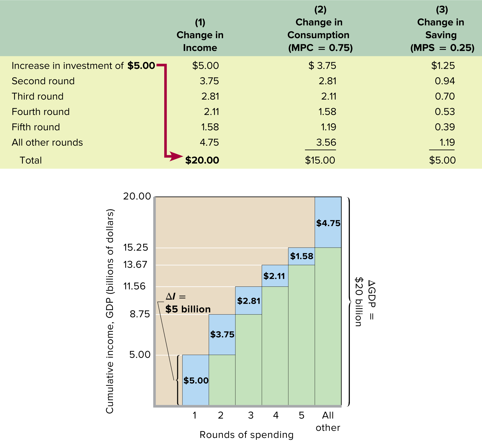
ex. refer to the below figure. investment spending increases by $5 billion and there is an MPC of 0.75.
Since any expenditure is received as income by someone else, there is a $5 billion increase in the incomes of households
Round 1: the $5 billion increase in income initially raises consumption by $3.75 (= 0.75 × $5) billion and saving by $1.25 (= 0.25 × $5) billion
Round 2: Other households receive as income the $3.75 billion of consumption spending and consume 0.75 of this $3.75 billion, or $2.81 billion, and save 0.25 of it, or $0.94 billion.
Round 3: The $2.81 billion that is consumed flows to still other households as income to be spent or saved. The process continues with the added consumption and income becoming less in each round.
The process ends when there is no more additional income to spend.
The Multiplier and the Marginal Propensities
The MPC and the multiplier are directly related and the MPS and the multiplier are inversely related.
Multiplier = 1 / (1-MPC)
Because MPC + MPS = 1,
Multiplier = 1 / MPS
The smaller the MPS, the greater the multiplier
this is b/c consumption is greater when saving is lesser
ex.
In the above figure, there is an initial $5 billion change in spending (investment in this case) an MPC of 0.75, and an MPS of 0.25
the multiplier = 1/0.25 = 4
if only the MPC is given, find the MPS by doing 1 - MPC
in the end, there was a total $5 billion * 4 = $20 billion increase in income
How Large Is the Actual Multiplier Effect?
In reality, consumption of domestic output (and therefore real GDP) increases in each round by a lesser amount than implied by the 1/MPS multiplier equation alone
Buying imports and paying taxes drains off some of the additional consumption spending on domestic output
Considering that increases in spending can drive up prices, an increase in spending may be partly dissipated as inflation rather than realized fully as an increase in real GDP.
Economists disagree on the size of the actual multiplier in the United States. Estimates range from 0-2.5.