AP Calculus AB - Ultimate Guide
Unit 1: Limits and Continuity
Limits
Limits are the value that a function approaches as the variable within the function gets nearer to a particular value.
We don’t really care what’s happening at the point, we care about what’s happening around the point
To find the limit of a simple polynomial, plug in the number that the variable is approaching
Ways to Find Limits
Look on a graph to see what it approaches
If the graph approaches two different values for the same number, the limit does not exist
Estimate from a table
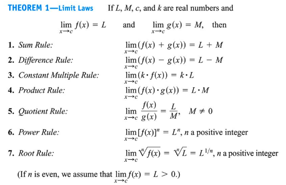
Algebraic Properties
Algebraic Manipulation
You can factor the numerator and denominator, then cancel any removable discontinuities
This is mostly useful if you get limits where the denominator is equal to 0
For example, (x+3)(x+2)/(x+3)(x-3)
(x+3) is able to be removed → removable discontinuity
Squeeze Theorem
Conditions
For all values of x in the interval that contains a, g(x) ≤ f(x) ≤ h(x)
g and h have the same limit as x approaches a
lim g(x) = L, lim h(x) = L, therefore lim f(x) = L
Trig limits as x approaches 0:
lim [sin(x)/x] = 1
lim [(cos(x)-1)/x] = 0
lim [sin(ax)/x] = a
lim [sin(ax)/sin(bx)] = a/b
Continuity
Jump Discontinuity
Occurs when the curve “breaks” at a particular place and starts somewhere else
The limits from the left and the right will both exist, but they will not match
Essential/Infinite Discontinuity
The curve has a vertical asymptote
Removable Discontinuity
An otherwise continuous curve has a hole in it
“Removable” because one can remove the discontinuity by filling the hole
Continuity Conditions
For f(x) to be continuous when x=c:
f(c) exists
the limit as x→c exists
lim f(x) = f(c)
x→c
A function is continuous on an interval if it is continuous at every point on that interval
Removing Discontinuities
You can remove a discontinuity by redefining the function without that point in the domain
This is frequently done by factoring out a common root between the numerator and denominator
Limits and Asymptotes
Vertical asymptote: a line that a function cannot cross because the function is undefined there
Horizontal asymptote: the end behavior of a function
A horizontal asymptote can be crossed
Horizontal Asymptote Rules
If the highest power of x in a rational expression is in the numerator, then the limit as x approaches infinity is infinity: there is no horizontal asymptote
If the highest power of x is in the denominator, then the limit as x approaches infinity is zero and the horizontal asymptote is the line y=0
If the highest power is the same, then the limit is the coefficient of the highest term in the numerator divided by the coefficient of the highest term in the denominator
Intermediate Value Theorem (IVT)
IVT - Guarantees that if a function f(x) is continuous on the interval [a,b] and C is any number between f(a) and f(b), ten there is at least one number in the interval [a,b] such that f(x) = C
Unit 2: Differentiation: Definition and Fundamental Properties
Rates of Change
We know that there are two ways of finding the rate of change
We can use the difference quotient to find the Average Rate of Change
The difference quotient is the rate of change over an interval of time
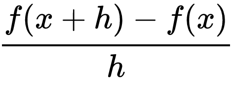
A simpler way of saying this is y2 - y1/x2-x1
The other way of finding the rate of change is at a specific point in time and this is called the Instantaneous Rate of Change
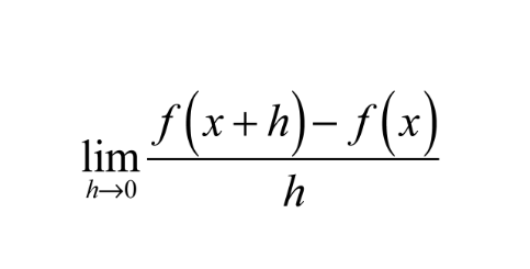
This is the difference quotient but with a limit as h → 0
Slopes of Lines & Definition of Derivative
Let’s say we had a line that isn’t linear, and we want to find the slope
For a linear line, the slope is “rise over run” but we can’t do that for a curved line
Therefore we have to use the secant line to approximate the slope
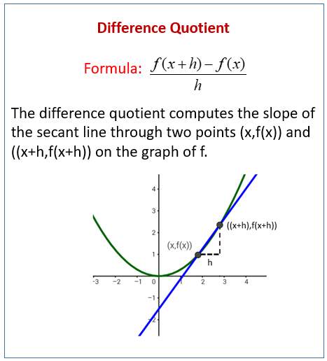
We can find the slope of the secant line using the difference quotient!
(Look at the formula above)
The closer the points are, the more accurate this slope will be
Therefore we can use a different kind of line- the tangent line- that touches the curve at exactly one point
We get this line by using the Instantaneous Rate of Change (remember: the difference quotient but with a limit as h → 0)
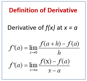
This is called the definition of the derivative!
Remember that the derivative is just the rate of change at a specific point, so we use a limit to find the slope as x gets infinitesimally small
Derivative Notation
Function: | First Derivative: | Second Derivative: |
|---|---|---|
f(x) | f’(x) | f'“(x) |
g(x) | g’(x) | g”(x) |
y | y’ or dy/dx | y” |
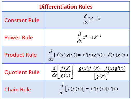
Derivative Rules
Using the limit definition of the derivative is tedious, so we have rules that can make taking a derivative easier!
Constant Rule: If f(x) = k where k is a constant then f’(x) = 0
Ex. f(x) = 10 so f’(x) = 0
Constant Multiple Rule: If you have a constant multiplied by a function, you can “pull the constant out”
So [k * f(x)]’ would be the same as k * f’(x)
The Power Rule: If f(x) = x^n then f’(x) = nx^n-1
For example x^4 becomes 4x^3 and 2x^2 would be 4x
A good way to describe this rule is to “multiply down and decrease the power”
The power rule works for polynomials!
The Product Rule: If you have two polynomials multiplied by each other like (2x +7)(9x + 8) you could multiply it out and then use the power rule, but this takes time, so we have something called the product rule.
The product rule says that if f(x) = uv then f’(x) = (u)(dv/dx) + (v)(du/dx)
You take the first term and multiply it by the derivative of the second term (using the power rule) then add that to the second term multiplied by the derivative of the first term
The way I learned it was “1d2 + 2d1” (first * derivative of second + second * derivative of the first)
The Quotient Rule: If you need to take the derivative of a fraction, you have to use this rule
The Quotient Rule says that if f(x) = u/v then f’(x) = (v)(du/dx) - u(dv/dx) / v^2
You take the denominator and multiply it by the derivative of the numerator, then subtract the numerator multiplied by the derivative of the denominator all over the denominator squared
The way I learned it was “low d high - high d low/ low^2” (low * derivative of high - high * derivative of low over low^2)
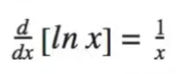
The last set of things that you have to know are “memory derivatives” or things that are easier to memorize than to derive. These will be the derivatives of sinx, cosx, e^x, and lnx

Unit 3: Differentiation: Composite, Implicit, and Inverse Functions
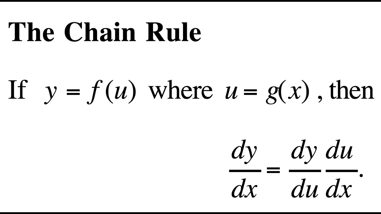
Chain Rule
When finding the derivative of a composite function, take the derivative of the outside function with the inside function g considered as the variable, leaving the “inside” function alone. Then we multiply this by the derivative of the inside function, with respect to the variable x.
The Chain Rule: If y = f(g(x)), then y’ = f’(g(x)) * g’(x) OR
If y = y(v) and v = v(x), then dy/dx = (dy/dv)*(dv/dx)
My personal memory trick for this is “douter, inner, dinner) → drop the power down to outside the parathesis, leave the inner, multiply by the derivative of the inner
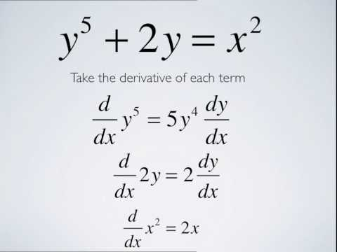
Implicit Differentiation
When you can’t isolate y in terms of x, you take the derivative implicitly. Essentially, you solve for the derivative of x with respect to y, in order to get a derivative in terms of both variables.
(dx/dy) = (1/(dy/dx))
Solving with the reciprocal allows to split up the variable and pair it to both sides, so that they can be factored.
You can also apply other, previous rules like the product rule in order to solve it. The AP exam loves to do this.
An easier way of describing implicit differentiation is that if your variable doesn’t match dx, then you need to follow it up with d(variable)/dx
For example, if we’re given x^2 + y^2 = 25 at the point (3, 4), we need to implicitly differentiate → doing this with respect to x we get:
2x + 2y(dy/dx) = 0
Then you have to solve for dy/dx
dy/dx = -x/y
At the point (3, 4), we have x = 3 and y = 4. Substituting these values, we get:
dy/dx = -3/4
So the slope of the tangent line is -3/4.
We also know that the point (3, 4) lies on the tangent line. Using the point-slope form of the equation of a line, we get:
y - 4 = -3/4(x - 3)
This is the equation of our tangent line
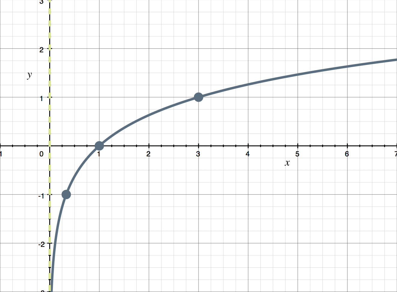
Inverse Function Differentiation
There is a simple formula in order to find the derivative of an inverse function.
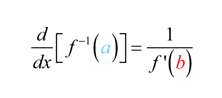
In short, we can find the derivative at a particular point by taking the reciprocal of the derivative at that point’s corresponding y value.
Say you want the derivative at the point (1,2) - you want g’(1). So find f’(2), then take the reciprocal - this is the value of g’(1).
Our original point is (1,2) so our reciprocal will be (2,1)
The same goes for our slope, find the slope at f’(2) and then take the reciprocal
Remember, f’(x) is the same as the slope!
The AP test usually only has 1-2 of these questions so don’t stress too much! 👍
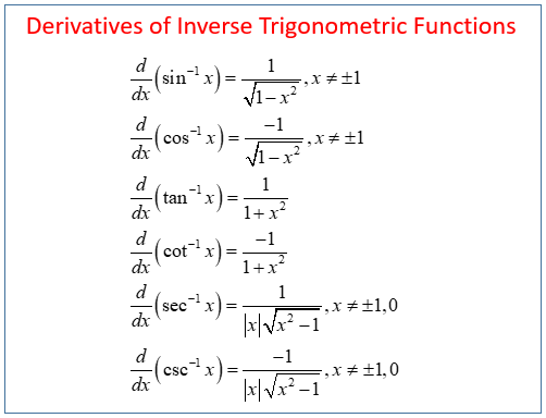
Inverse Trigonometry
This is going to be one that is easier to just memorize, but you can also find them by following the formulas explained in implicit differentiation and using trigonometry rules.
HINTS
When two terms are multiplied together, use product rule unless it’s easier to multiply it out
If you see a function within another function, you will almost certainly have to use chain rule
If there are x and y terms mixed together, we will need to use implicit differentiation
If you’re finding the derivative at a point, just plug it in and avoid the solving out
When evaluating derivatives at a point, look to see if the terms become one or zero
You can mentally take certain derivatives
If it is required to take a second derivative, simplify the first derivative before you start
Unit 4: Contextual Applications of Differentiation
Interpreting the Derivative
The derivative tells us the slope of the line tangent to the graph- which tells us the slope of the line at a particular point
This means that they can tell us the change of a unit over time. This will make sense with straight line motion.
Straight Line Motion
We know that position is measured in meters
We know that velocity is measured in meters per second (m/s)
Therefore we can derive position to get the rate of change- ie. meters per second!
We know that acceleration is measured in meters per second squared (m/s^2)
So we can derive velocity to get the rate of change- ie. meters per second per second!
You can also take the second derivative of position to get acceleration
Position: | x(t) (sometimes wrote as s(t)) | Meters |
|---|---|---|
Velocity: | x’(t) or v(t) | Meters/Second |
Acceleration: | x”(t) or v’(t) or a(t) | Meters/Second^2 |
Particles will speed up when the sign of velocity and acceleration match
The must both be negative or positive
For example, if a particle moves along a straight line with velocity function v(t) = 3t^2 - 4t + 2. Find the acceleration of the particle at time t=2?
Solution: The acceleration of the particle is the derivative of its velocity function. Thus, we take the derivative of v(t) with respect to t
a(t) = d/dt v(t) = 6t - 4
To find the acceleration at t=2, we substitute t=2 into the expression for a(t):
a(2) = 6(2) - 4 = 8
Non-Motion Changes
The derivative can also tell us the change of something other than motion
For example, let’s say the volume of water in a pool is equal to V(t) = 8t^2 -32t +4
Where V is the volume in gallons and t is the time in hours
If we want to find the rate that the volume of water is increasing we take the derivative
dV/dt = 16t - 32 gallons per hour
At t=2 the volume isn’t changing (equation equals 0)
Therefore it is increasing for all values >0
Another example would be where temperature of a cup of coffee is given by the function x(t) = 70 + 50e^(-0.1t), where t is the time in minutes since the coffee was poured. And we need to find the rate of change of the temperature with respect to time at t=5 minutes.
d/dt of x(t) = -5e^(-0.1t)
Evaluating this derivative at t=$ minutes, we get:
x’(5) = -5e^(-0.1(5)) ≈ -2.27
Related Rates
We just saw how the derivative can tell us the change of something but we can also have problems where the change of one thing is related to another- Related Rates!
Let’s say that a pool of water is expanding at 16π square inches per second and we need to find the rate of the radius expanding when the radius is 4 inches
We know that we can find the radius using A = πr^2
Now let’s relate our rates!
dA/dt = 2πr(dr/dt)
Notice how we had to follow r with dr/dt, this is because the change in R doesn’t match the change in A (implicit differentiation)
Now we have the change of the area (dA/dt) and the change of the radius (dr/dt)
Now we can plug in and solve!
16π = 2π(4)dr/dt
dr/dt = 2
The radius is changing at a rate of 2 inches per second
Let’s say a spherical balloon is being inflated at a rate of 10 cubic inches per second. How fast is the radius of the balloon increasing when the radius is 4 inches?
We know that the volume of a sphere is given by the formula V = (4/3)πr^3.
Differentiating both sides with respect to time t, we get:
dV/dt = 4πr^2 (dr/dt)
We are given that dV/dt = 10 cubic inches per second and r = 4 inches. Substituting these values, we get:
10 = 4π(4^2)(dr/dt)
Simplifying, we get:
dr/dt = 10/(16π)
Therefore, the radius of the balloon is increasing at a rate of 10/(16π) inches per second when the radius is 4 inches.
To solve related rates problems in calculus, follow these steps:
Read the problem carefully and identify all given information.
Draw a diagram if possible.
Determine what needs to be found and assign a variable to it.
Write an equation that relates the variables involved.
Differentiate both sides of the equation with respect to time.
Substitute in the given values and solve for the unknown rate.
Remember to always include units in your final answer and to check that your answer makes sense in the context of the problem.
Linearization
Differentials are very small quantities that correspond to a change in a number. We use Δx to denote a differential.
They can approximate the value of a function!
Remember the limit definition of a derivative?
We just have to replace h with Δx and remove the limit!
We get that f(x + Δx) ≈ f(x) + f’(x)Δx
This is no longer equal to the derivative, but an approximation of it
In simple terms “the value of a function (at x plus a little bit) is equal to the value of the function (at x) plus the product of the derivative of the function (at x) plus a little bit”
Let’s say we needed a differential to approximate (3.98)^4
We have to let f(x) = x^4, x= 4, and Δx = -0.02
Now we have to find f’(x) which is 4x^3
Now plug into f(x + Δx) ≈ f(x) + f’(x)Δx
(x + Δx)^4 = x^4 + 4x^3Δx
When we plug in x= 4 and Δx= -0.02 we get 250.88
You can check this using your calculator!
L’Hospital’s Rule
If a limit gives you 0/0 or ∞/∞, then it is called “indeterminate” and you can use
L’Hospital’s Rule to interpret it!
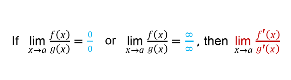
L’Hospital’s Rule says that we can take the derivative of the numerator and denominator and try again
Let’s say we have the limit of 5x^3 -4x^2 +1/7x^3 +2x - 6 as it approaches infinity
This equals ∞/∞ so we can take the derivative of the top and bottom
Then we get 15x^2 -8x/21x^2 +2
This is still ∞/∞ so we take the derivative again
Then we get 30x -8/42x which is still ∞/∞
We take the derivative to get 30/42 or 5/7 which is our answer!
Unit 5: Analytical Applications of Differentiation
The Mean Value Theorem (MVT)
The MVT links the average rate of change and the instantaneous rate of change
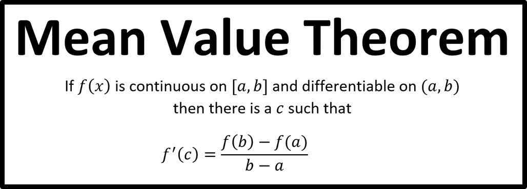
There must be some point in the interval where the slope of the tangent line equals the slope of the secant line (that connects the endpoints)
Rolle’s Theorem is a special case of the MVT
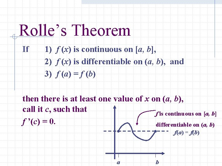
It means that a continuous, differentiable curve has a horizontal tangent between any two points
Extreme Value Theorem
The Extreme Value Theorem states that if a function is continuous on a closed interval, then it must have both a maximum and a minimum value on that interval.
The maximum and minimum are called extrema and there are two types of each:
Absolute (global) → No other value is higher/lower than an absolute
Local (relative) → The highest/lowest in the nearby area
Any place an extrema could exist are called critical points
Intervals of Increase and Decrease
Using the first derivative we can identify when the original function is increasing or decreasing
For all the values that f’(x) > 0, the function is increasing
For all the values that f’(x) < 0, the function is decreasing
Take the derivative of the function
Set it equal to zero to find your critical numbers
Plug in a number above the critical point and below the critical point to find the sign of f’(x)
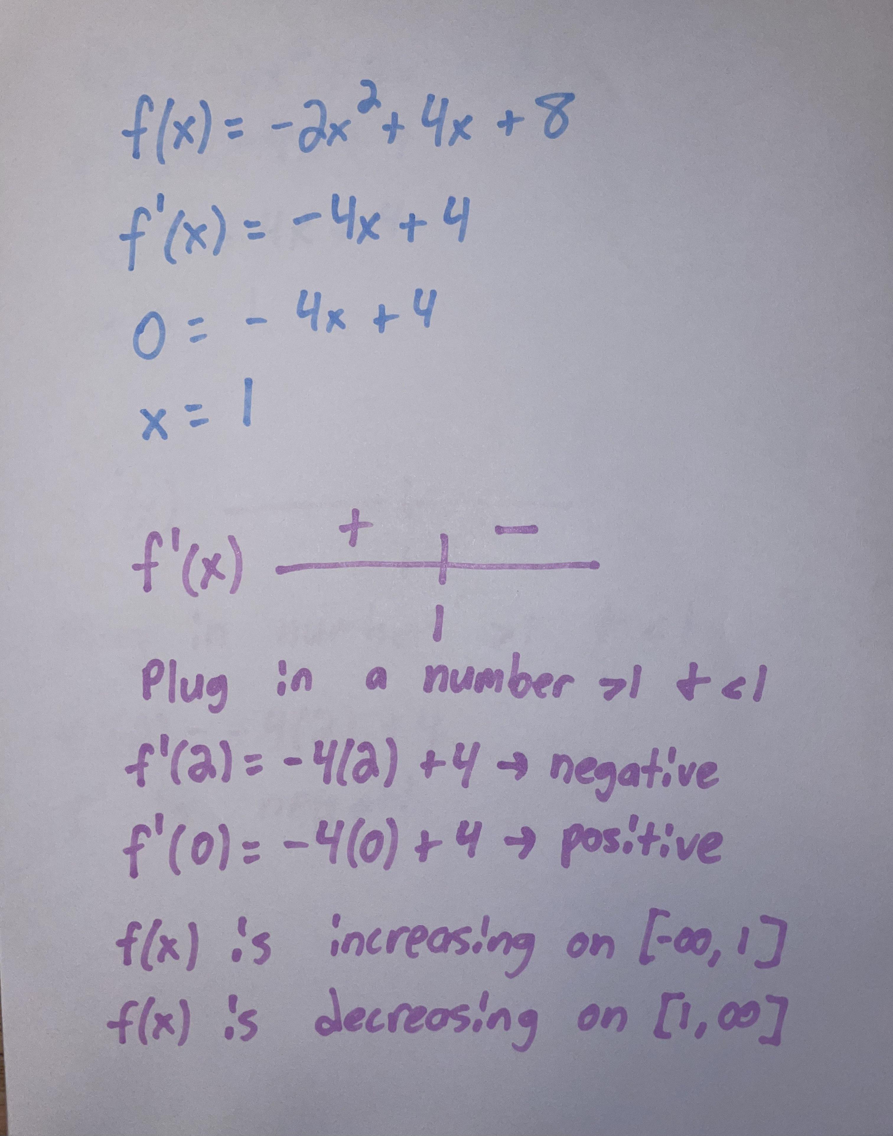
In this example we can see that if we plug in a number higher than 1 (such as 2) we get a negative number → f(x) is decreasing
If we plug in a number less than than 1 (such as zero) we get a positive number → f(x) is increasing
Let’s say that we are given the function f(x) = x^3 - 6x^2 + 9x + 2, and we need to find where the function is increasing or decreasing.
To solve this problem, we need to take the derivative of the function f(x) and set it equal to zero to find the critical points.
f'(x) = 3x^2 - 12x + 9
Setting f'(x) equal to zero, we get:
3x^2 - 12x + 9 = 0
Solving for x, we get:
x = 1 or x = 3
Now, we need to determine whether the function is increasing or decreasing on each interval between the critical points. We can do this by plugging in test values into f'(x) and seeing if the result is positive or negative.
When x < 1, f'(x) is negative, so the function is decreasing.
When 1 < x < 3, f'(x) is positive, so the function is increasing.
When x > 3, f'(x) is negative, so the function is decreasing.
Therefore, the function f(x) is increasing on the interval (1, 3) and decreasing on the intervals (-∞, 1) and (3, ∞).
Relative Extrema
The first derivative also tells us relative maxima and minima of a function
When the first derivative shifts from positive to negative there will be a relative maximum
When the first derivative shifts from negative to positive there will be a relative maximum
For example, our function above has a relative maximum at x=1 because our derivative changes from positive to negative
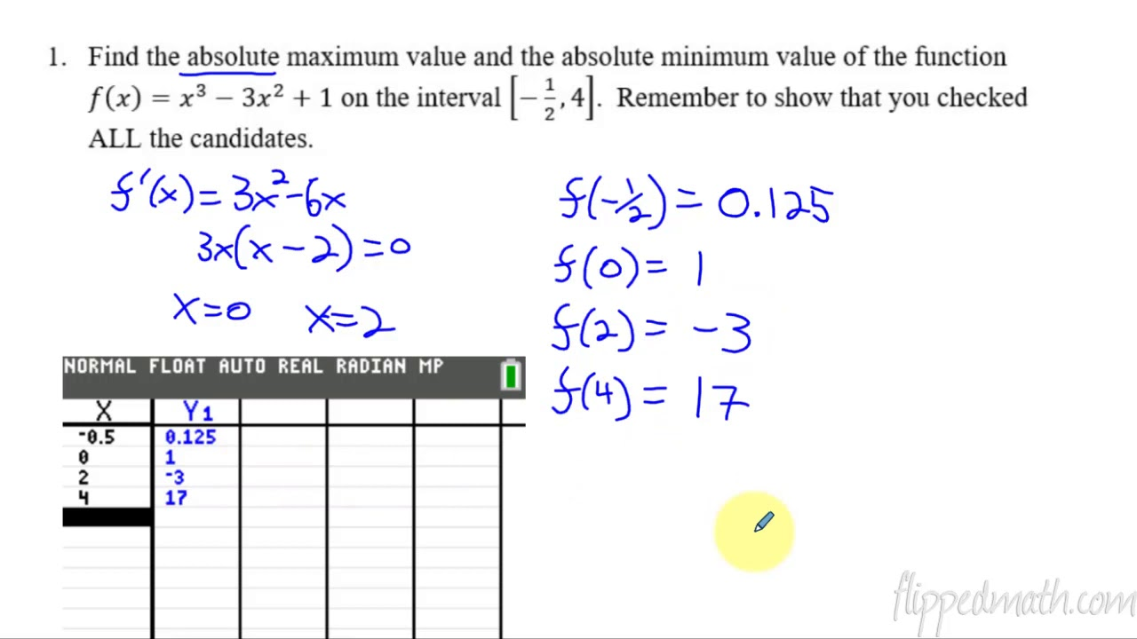
Candidate’s Test & Absolute Extrema
To find the absolute (global) extrema you have to consider the endpoints and critical numbers
Make a table of these values
Then plug back into your ORIGINAL FUNCTION
Function Concavity
The first derivative tells us if the function is increasing or decreasing
The second derivative tells us if this is happening at an increasing or decreasing rate
This is given to us by something called concavity
For all the values that f”(x) > 0, the function is concave up
For all the values that f”(x) < 0, the function is concave down
Take the second derivative of the function
Set it equal to zero to find your points of inflection
Points of inflection are where the second derivative changes sign
Plug in a number above the critical point and below the critical point to find the sign of f”(x)
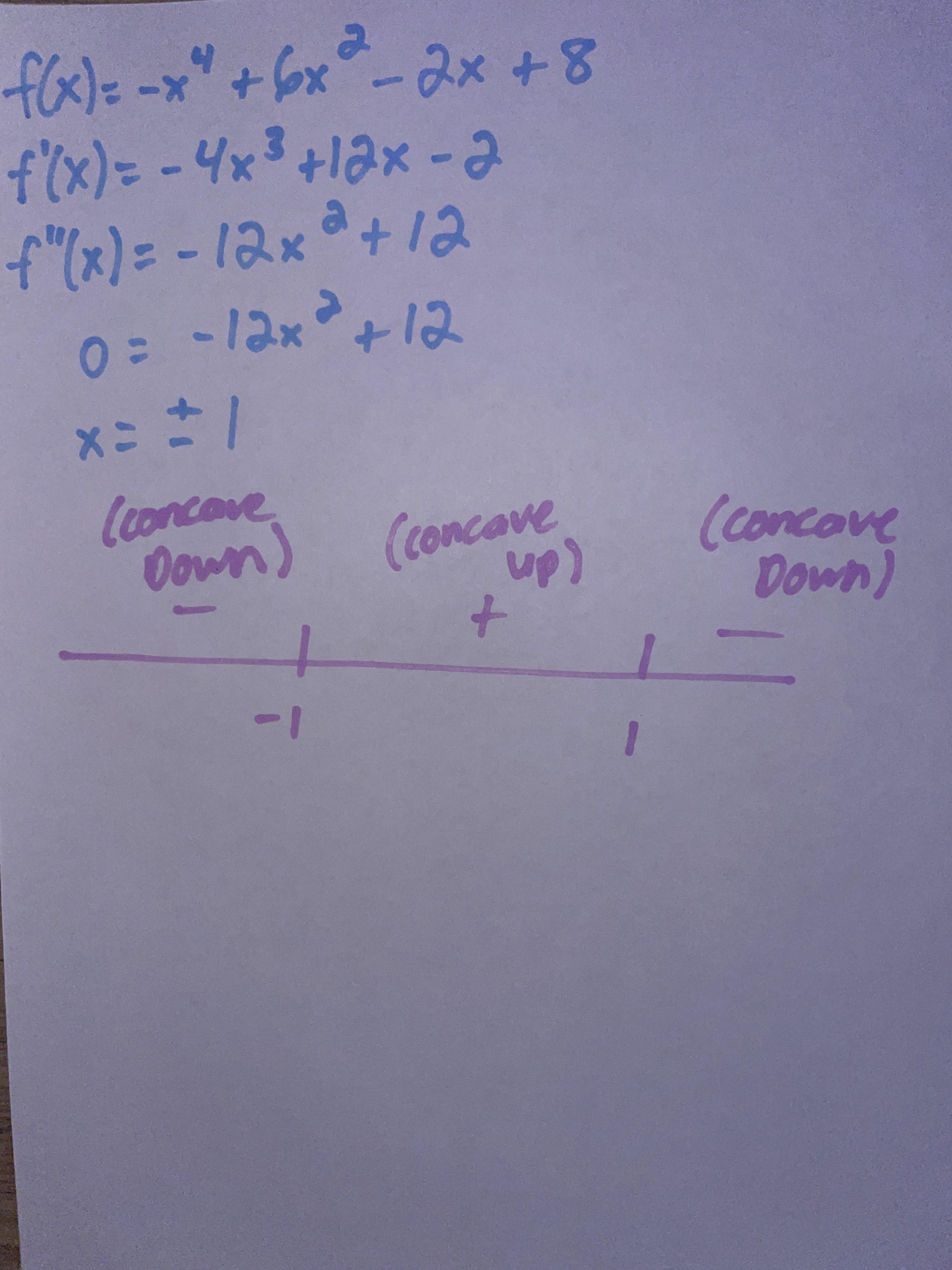
Suppose we have a function f(x) = x^3 - 6x^2 + 9x + 2. Find the intervals where the function is concave up or concave down using the second derivative test.
To find the intervals where the function is concave up or down, we need to take the second derivative of f(x).
f(x) = x^3 - 6x^2 + 9x + 2
f'(x) = 3x^2 - 12x + 9
f''(x) = 6x - 12
To find the critical points, we set f''(x) = 0:
6x - 12 = 0
x = 2
Now we can use the second derivative test to determine the intervals of concavity:
When x < 2, f''(x) < 0, so the function is concave down.
When x > 2, f''(x) > 0, so the function is concave up.
Therefore, the function is concave down on the interval (-∞, 2) and concave up on the interval (2, ∞).
Unit 6: Integration and Accumulation of Change
The Integral & Area Under A Curve
Up to here we’ve learned about the derivative, the rate of change. Now we have the integral ∫ also called the antiderivative.
The derivative shows us the change/unit
So the antiderivative shows us the total change
The first type is called a definite integral and shows us the area of the region under the function and the x-axis. It gives us the accumulation/total change!
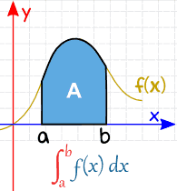
Let’s say we have a function that is shaped like that (or any function at all), if the definite integral needs us to get the area under the function, how would we do that?
Because this is a shape that we have no formula for, we can estimate it using shapes that we do know
We can split this area up into rectangles!
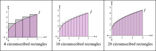
The more rectangles we have, the better our estimate is!
This method is called a Riemann sum!
Riemann & Trapezoidal Sums
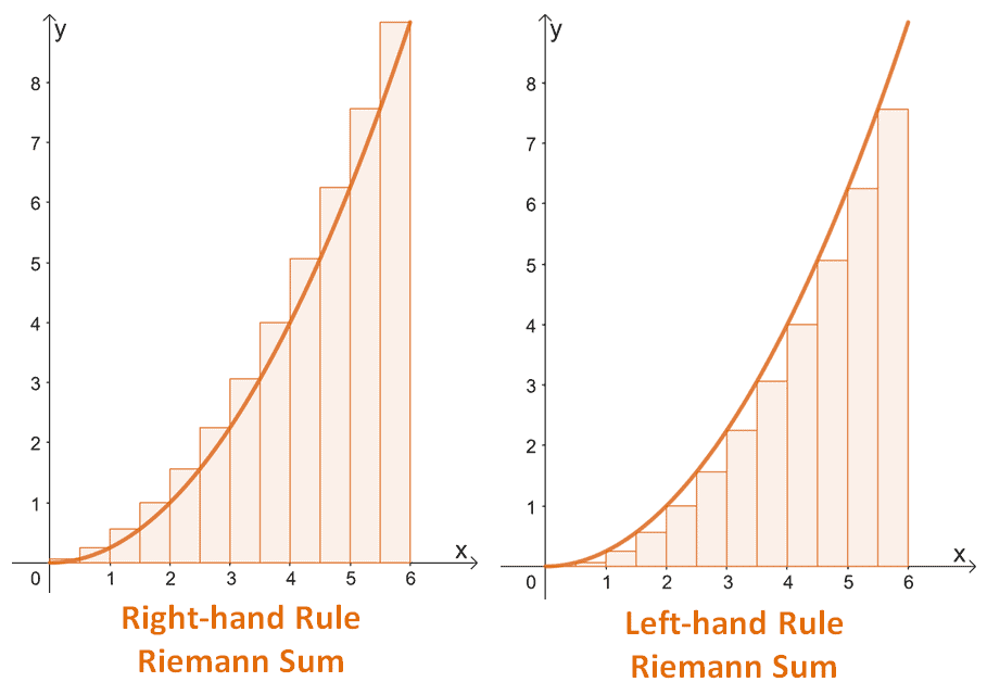
We can take a Riemann Sum from the left, or from the right!
For left-handed sums we use the endpoints (number) on the left
For right-handed sums we use the endpoints (number) on the right!
The formulas are the same for any rectangle, base * height!
Take the width of your rectangle and multiply it by the height of the rectangle!
Do this for each rectangle you have and add them all together
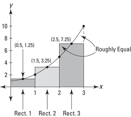
To get these rectangles even more accurate, we can use a midpoint sum
We still use the formula for a rectangle, but we use the value for the height in between!
A shape that would more closely fit the shape of the curve is a trapezoid
Therefore, we can use trapezoidal sums!
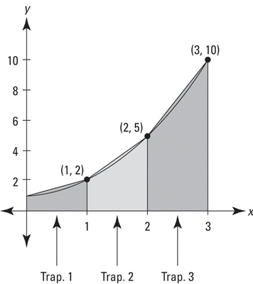
We know that the formula for a trapezoid is (1/2)(b1 + b2)(h)
For example, our second trapezoid would be (1/2)(2 + 5)(1)
Still a width of 1 but we add the two heights!
Most of the time you are given a table to take a Riemann Sum from!
0 | 2 | 4 | 7 |
|---|---|---|---|
1 | 6 | 10 | 15 |
Left Sum: (2)(1) + (2)(6) + (3)(10)
Notice how this is a left sum so we don’t use the furthest right value
Right Sum: (2)(6) + (2)(10) + (3)(15)
Same thing for the right, except we don’t use the furthest left value
Midpoint: (4)(6)
Not complete but you see how we use a width of 4 and then the height in between
Trapezoid: (1/2)(1+6)(2) + (1/2)(6+10)(2) + (1/2)(10+15)(3)
Tabular Riemann Sums
The majority of the time when you have to use a Riemann Sum, the AP gives it to you in tabular format
Years:(t) | 2 | 3 | 5 | 7 | 10 |
|---|---|---|---|---|---|
Height:H(t) | 1.5 | 2 | 6 | 11 | 15 |
Trapezoids: (1/2)(1.5+2)(1) + (1/2)(2+6)(2) + (1/2)(6+11)(2) + (1/2)(11+15)(3)
Left Sum: (1)(1.5) + (2)(2) + (2)(6) + (3)(11)
Right Sum: (1)(2) + (2)(6) + (2)(11) + (3)(15)
You do not have to simplify these!
Fundamental Theorem of Calculus & Antiderivatives
For differentials, you know that you had a set of different rules that you can use to take the derivative. The same applies for the antiderivative!
Intuitively, it’s the opposite of what you do to take a derivative EXCEPT…
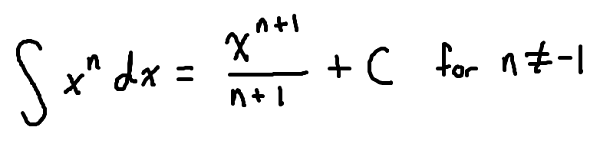
We can only use the power rule!
If the power rule for a derivative tells us to multiply down and decrease the power, then the opposite of that would be to divide and increase the power!
The +C is very important!
If you take the derivative of any number without an x, you get zero
Therefore if we’re doing the reverse process, we don’t know what this number could be, therefore we add on a C for the constant of integration
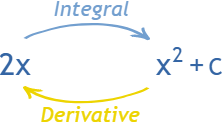
The integral of 2x is really 2x^2/2 but that simplifies to x^2!
Remember that if the integral is not in power rule format, we must algebraically manipulate it so that we can use the power rule
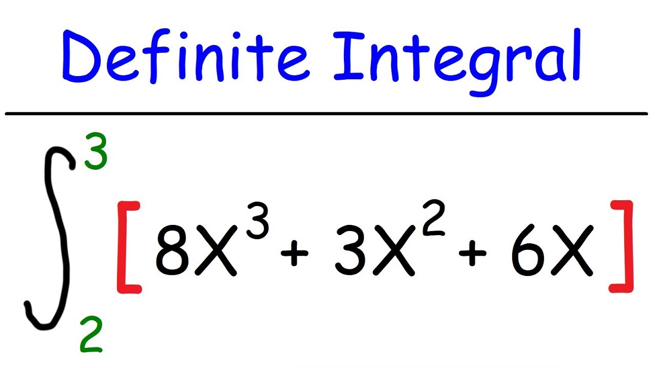
The two numbers at the top and bottom of the integral means that it is a definite or bounded integral
It means we are trying to find the area below 2 and 3
Because we have a function, we don’t have to graph it out, instead we have something called the First Fundamental Theorem of Calculus
(8 chapters in and you’re just now learning about the thing fundamental to calculus huh)
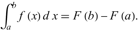 The first fundamental theorem says that the integral from a to b is equal to the antiderivative, plug in b, and then plug in a and subtract!
Let’s say that we had ∫2x from before (from x=2 to x=3), according to the first fundamental theorem it is equal to (3)^2 - (2)^2
Advanced Integration
Sometimes, getting an integral into power rule format is nearly impossible, in those cases there are other techniques we can do!
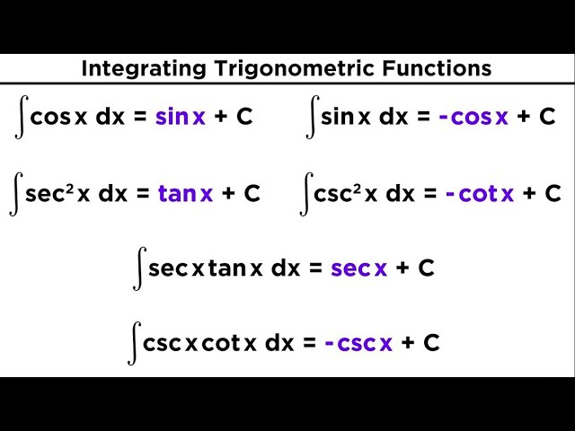
If your integral contains trigonometry, the best thing to do is just memorize the derivative of trig functions, and the integral will be the opposite
Ex. d/dx sinx = cosx
Therefore, ∫cosx = sinx
You can manually derive these but because this is a timed AP exam it’s more efficient to memorize these!
Your other option is U-substitution!
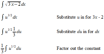
Chose a term to be your “u”
Take the derivative of this value to get du/dx
Substitute in your u value for the term and your du/dx value for dx
Take the integral
U-substitution is tricky but helpful for some problems!
You got this!!! 👍
Ex. ∫(x - 4)^10
Let u = x-4
du/dx = 1
dx = du/1
∫(u)^10 du
u^11/11 + C
(x-4)^11/11 + C
Unit 7: Differential Equations
Introduction & Slope Fields
In related rates we saw how we can model the change in one thing related to another with derivatives, and differential equations are similar!
Oftentimes, variables are not constant, so we have to represent their change using a derivative (Ex. the change in y is dy/dx)
A differential equation models the change in one variable with respect to another
Slope fields show us what the slopes look like at points on a graph
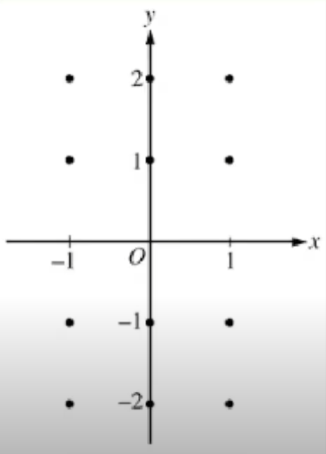
This is for the equation dy/dx = x
Remember that this is a derivative so it will show us the slope at these points!
All you have to do to construct a slope field is plug in your x/y (or both) values into your differential equation and draw that as your slope
Ex. The slope at x = -1 would be -1 (because dy/dx = x)
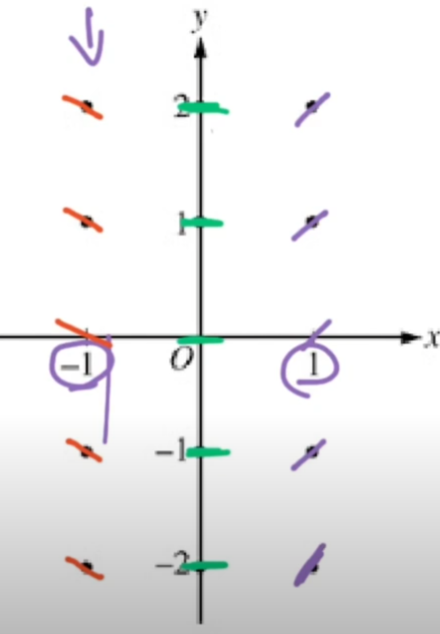
The AP exam might also require you to sketch a solution curve given a slope field!
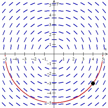
All you have to do is “flow” with the slopes
Make sure you don’t cross abruptly or draw a line that doesn’t follow the slope
Because this is by hand, it doesn’t have to be exact, just try and go with the tangent lines!
Differential Equations
If you’re given a differential equation where the derivative of a function is equal to some other function, you have to solve for the original! You can do this by taking the integral (antiderivative) of both sides!
A good memory trick is that differential equation problems will be SIPPY problems
S: separate (dy and dx on separate sides)
I: integrate (remove the derivative)
P: Plus C (add your c value to your integral)
P: Plug in your initial condition
Y: Y equals (solve to find what y is)
Example: If dy/dx = 4x/y and y(0) = 5 we need to solve for y
Start by separating → ydy = 4xdx
Then integrate → ∫ydy = ∫4xdx → y^2/2 = 2x^2 + C
(Make sure you add C!)
Plug in → (5)^2/2 = 2(0)^2 + C
C = 25/2
Now set y equals → y = 2x^2 + 25/2
Unit 8: Applications of Integration
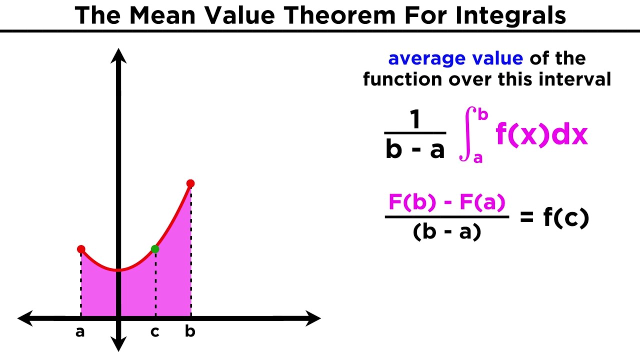
Average Value of Functions
Remember that to calculate the average we add everything up and then divide!
The integral is the summation of everything, so we can use it to find the average of a function!
The only thing we have to change is by dividing our integral!
For example, if we had the interval 0 to 40, we can take the integral of our function and divide it by our interval! So it would be 1/40 * ∫f(x)
Position, Velocity, and Acceleration
Similar to how we can go from position → velocity using the derivative, we can do the reverse using the integral!
Displacement | ∫v(t) |
|---|---|
Position | ∫|v(t)|(Absolute value) |
Velocity | ∫a(t) |
Remember that the FTC still applies, for example velocity will be equal to ∫a(t) from a to b which is: ∫a(t) = v(b) - v(a)
Area Between Two Curves
The integral gives us the area below a function
Therefore, we can subtract the area of one function and another to get the area between the two!
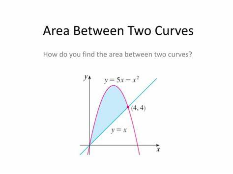
Finding this area is pretty simple, all we have to do is integrate the top function & subtract the bottom function!
We need to take the integral from where the functions start (normally zero) to where they intersect
For the problem we would have ∫5x-x^2 from 0 to 4 - ∫x from 0 to 4
Most all problems for area between two curves will be similar to this
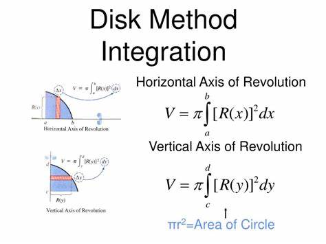
Volume by Cross Sectional Area
We get a 2D shape from the area under a curve, if we rotate this shape → we get a 3D object
To find the area we just integrate the volume formula!
What is the formula for finding the volume of a shape using integrals?
To find the volume of a shape using integrals, we use the formula for the cross-sectional area (length times width) and multiply it by the height, which is represented by the variable "dx" in the integral. Therefore, the formula for the volume of a rectangular shape using integrals is:
V = ∫(length x width) dx
where V is the volume, and the integral is taken over the range of the height of the shape.
That would give us the volume for a rectangle (because their area is just l * w)
The majority of the time, when we are integrating a curve, we get discs or circles
Therefore, we can almost always use the disc method to find our volume
We know that the area of a circle is πr^2
So using our integral we would have V = ∫πr^2
You can combine this with area between two curves problems and have ∫πR^2 - ∫πr^2]