


Chapters 25.1-25.5: Aggregate Expenditures Model
Assumptions and Simplifications
Assumptions of the aggregate expenditures model created by Keynes reflect the economic conditions of the Great Depression:
the main assumption is that prices in the economy are fixed (stuck rather than sticky)
actual prices did not fall sufficiently during the Great Depression, and the economy sank far below its potential output
As households and businesses greatly reduced their spending, inventories of unsold goods rocketed. Firms will unable or unwilling to slash their prices, so they reduced their current production. This meant discharging workers, idling production lines, and even closing entire factories.
US real GDP fell by 27% from 1929-1933
unemployment rate reached 25%
assume that unless specified otherwise, the presence of excess production capacity and unemployed labor implies that an increase in aggregate expenditures will increase real output and employment without raising the price level
assume that the total amount of spending is the primary factors that determines the amount of real GDP produced
The Keynesian aggregate expenditures model is still insightful even today because many prices in the modern economy are inflexible downward over relatively short periods of time.
Consumption and Investment Schedules
private closed economy::
the two components of aggregate expenditures are consumption, C, and gross investment, Ig.
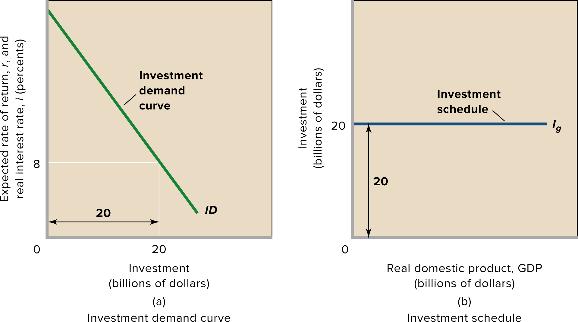
To add the investment decisions of businesses to the consumption plans of households (consumption schedule), we need to construct an investment schedule showing planned investment at each possible level of GDP.
this is not the same as the investment-demand curve
planned investment::
The amount that firms plan or intend to invest.
assume that this planned investment is independent of the level of current disposable income or real output.
the interest rate and investment demand curve determine the constant amount of investment ($20 billion in the example below)
Equilibrium GDP
aggregate expenditures schedule::
A table of numbers showing the total amount spent on final goods and final services at different levels of real gross domestic product (real GDP).
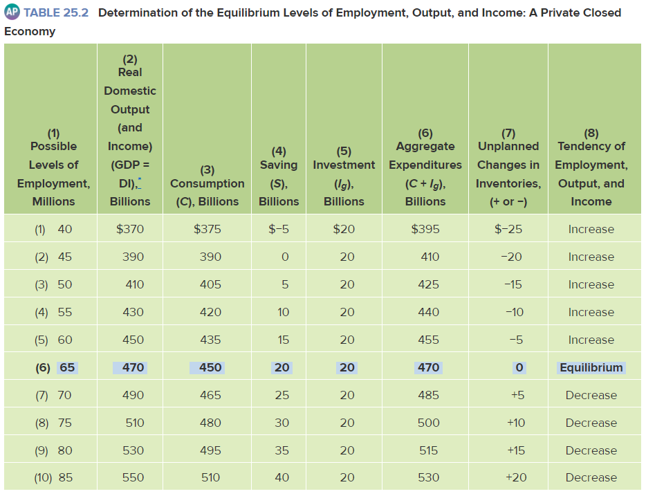
We are working with planned investment—see the data in column 5 . These data show the amounts firms plan or intend to invest, not the amounts they actually will invest if there are unplanned changes in inventories.
Equilibrium GDP::
the level at which the total quantity of goods produced (GDP) equals the total quantity of goods purchased
In a private closed economy, the equilibrium GDP is where C + Ig = GDP
Disequilibrium
No level of GDP other than the equilibrium level of GDP can be sustained
If spending exceeds GDP produced
Because buyers would be taking goods off the shelves faster than firms could produce them, an unplanned decline in business inventories will occur (column 7 of aggregate expenditures schedule)
Businesses will increase production
Greater output will increase employment and total income until the equilibrium level of GDP is reached.
If produced GDP exceeds spending
An unplanned increase in business inventories will occur. Being unable to recover the costs of producing output that isn’t purchased, businesses will cut back on production. The resulting decline in output would mean fewer jobs and a decline in total income.
Graphical Analysis

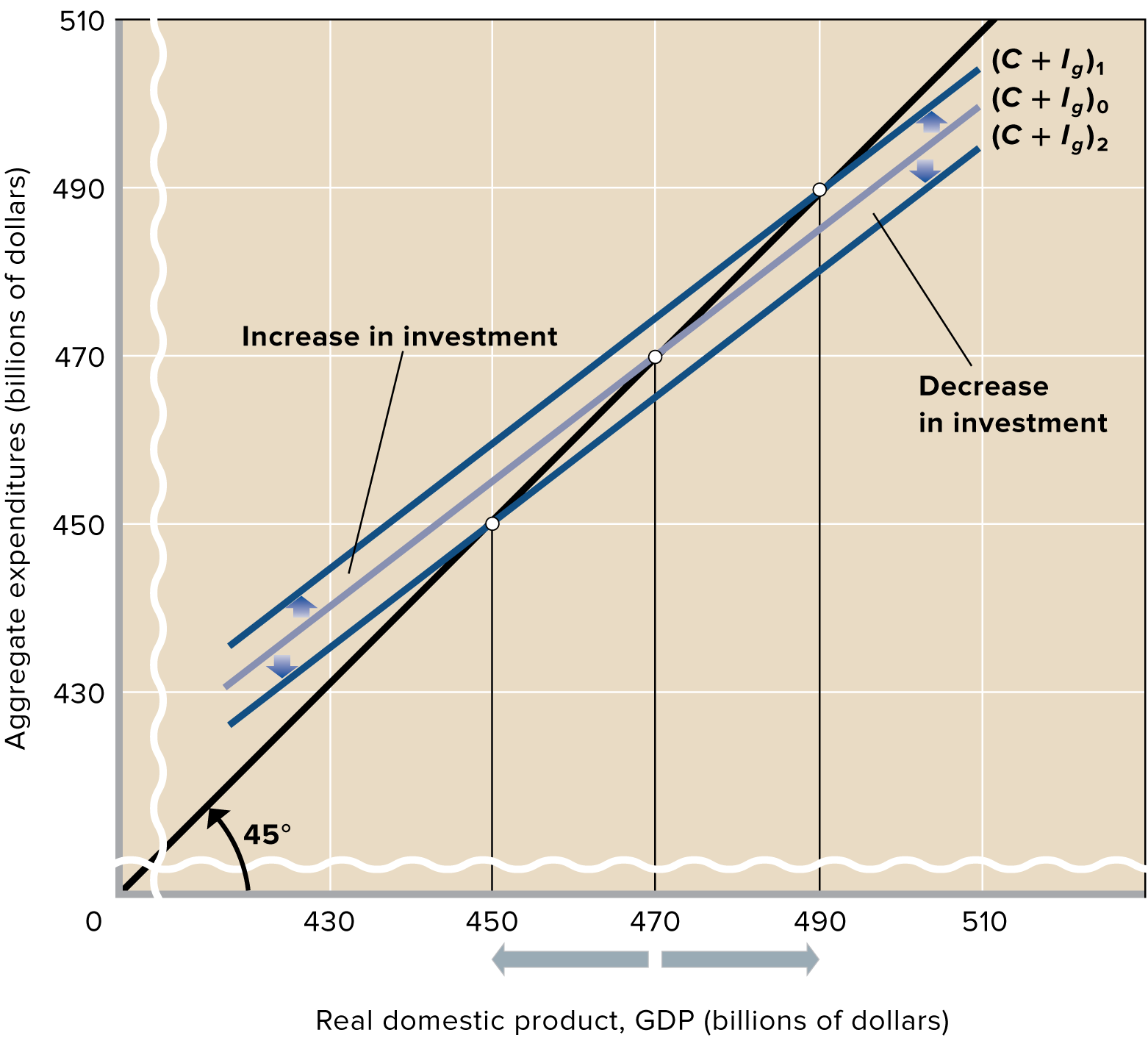
the aggregate expenditures line C + Ig shows that total spending (y-value) rises with income and output (x-value), but not as much as income and output (x-value) rises
because the aggregate expenditures line C + Ig is parallel to the consumption line C, the slope of the aggregate expenditures line = slope of line C = MPC
The equilibrium level of GDP is determined by the intersection of the aggregate expenditures schedule and the 45° line.
locates the only point at which aggregate expenditures (on the vertical axis) are equal to GDP (on the horizontal axis).
Production exceeds spending to the right of the equilibrium point
Spending exceeds production to the right of the equilibrium point
Other Features of Equilibrium GDP (closed private economy where C + Ig = GDP)
Saving Equals Planned Investment
leakage::
A withdrawal of potential spending from the income-expenditures stream via saving, tax payments, or imports
Saving is a leakage or withdrawal of spending from the economy’s circular flow of income and expenditures. It’s what causes consumption to be less than total output or GDP.
Therefore, consumption by itself is insufficient to remove domestic output from the shelves
Some of the output firms produce will be capital goods sold to other businesses.
Investment—the purchases of capital goods—is therefore an injection of spending into the income-expenditures stream. As an adjunct to consumption, it is a potential replacement for the leakage of saving.
Injection::
An addition of spending into the income-expenditure stream: any increment to consumption, investment, government purchases, or net exports.
If saving at a certain level of GDP exceeds investment, then C + Ig will be less than GDP.
This is an above-equilibrium GDP. Excess saving, or spending deficiency, will reduce real GDP.
if the injection of investment exceeds the leakage of saving, then C + I will be greater than GDP.
This is a below-equilibrium GDP. Excess spending drives GDP higher.
Only where S = Ig will aggregate expenditures (C + Ig) equal real output (GDP)
No Unplanned Changes in Inventories
there are no unplanned changes in inventories at equilibrium GDP in a private closed economy
unplanned changes in inventories::
Changes in inventories that firms did not anticipate; changes in inventories that occur because of unexpected increases or decreases of aggregate spending (or of aggregate expenditures).
Unplanned inventory change = saving (S) - investment (Ig)
Equilibrium occurs only when planned investment and saving are equal. But when unplanned changes in inventories are considered, investment and saving are always equal, regardless of the level of GDP.
That is true because actual investment consists of planned investment and unplanned investment (unplanned changes in inventories)
Changes in Equilibrium GDP and the Multiplier
Recall that multiplier = 1/MPS or change in output/change in spending
If expected rate of return on investment rises or that the real interest rate falls such that investment spending increases, there would be an upward shift of the investment schedule (which is a horizontal line and not the ID curve).
In the figure, the $5 billion increase of investment spending will increase aggregate expenditures and raise equilibrium GDP by the multiplier (4) * the increase in investment ($5 billion) = $20 billion.
If the economy starts at (C + Ig)0, a $5 billion increase in spending will shift it to (C + Ig)1 but increase equilibrium real GDP from $470 billion to $490 billion because of the multiplier
If the expected rate of return on investment decreases or if the real interest rate rises, investment spending will decline and show a downward shift of the investment schedule and a downward shift of the aggregate expenditures schedule and decrease equilibrium GDP.
Adding International Trade
We move from a private closed economy to a private open economy that incorporates exports (X) and imports (M).
Net Exports and Aggregate Expenditures
To correctly measure aggregate expenditures for domestic goods and services, we must subtract expenditures on imports from total spending to get net exports.
net exports = exports - imports
in notation, Xn = X - M
For a private closed economy, aggregate expenditures are C + I
But for an open economy, aggregate expenditures are C + Ig + (X − M) or C + Ig + Xn
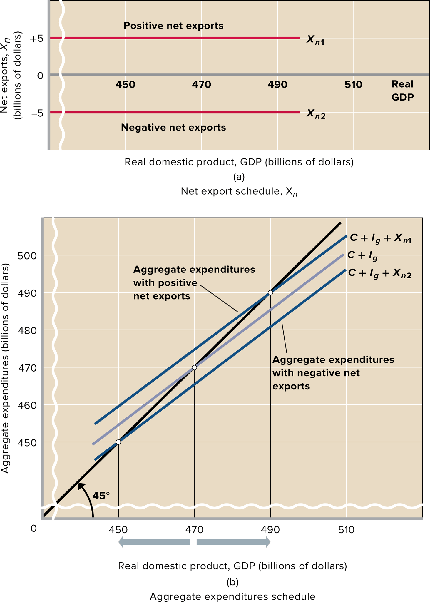
The Net Export Schedule
A net export schedule lists the amount of net exports that will occur at each level of GDP
We assume that net exports are independent of GDP whether they’re positive or negative
Net Exports and Equilibrium GDP
Positive net exports
exports exceed imports
ex. in the above figure, C + Ig shifts up to C + Ig + Xn1
Adding net exports of $5 billion has increased GDP by $20 billion, in this case implying a multiplier of 4.
Negative net exports
imports exceed exports
ex. in the above figure, C + Ig shifts down to C + Ig + Xn2
Subtracting net exports of $5 billion has decreased GDP by $20 billion, in this case implying a multiplier of -4 (or a multiplier of 4 in the opposite direction)
What circumstances or policies abroad affect US GDP?
Prosperity Abroad
A rising level of real output and income among U.S. foreign trading partners enables them to buy more US goods, thus raising U.S. net exports and increasing U.S. real GDP (assuming initially there is excess capacity to sell to them)
Exchange Rates
If the dollar is depreciated relative to other currencies
The price of U.S. goods in terms of those currencies will fall, stimulating purchases of U.S. exports.
U.S. customers will find they need more dollars to buy foreign goods and will also reduce their spending on imports.
Appreciation of the dollar would have opposite effects on net exports and equilibrium GDP
A Caution on Tariffs and Devaluations
Countries often look for ways to reduce imports and increase exports during recessions or depressions
A recession might tempt the U.S. federal government to increase tariffs and devalue the international value of the dollar (say, by supplying massive amounts of dollars in the foreign exchange market) to try to increase net exports.
But when we restrict our imports to stimulate our economy, we depress the economies of our trading partners.
They are likely to retaliate against us by imposing tariffs on our products. If so, our exports to them will decline and our net exports may in fact fall
This happened in the Great Depression
Some nations tried to increase their net exports by devaluing their currencies. Other nations simply retaliated by devaluing their own currencies.
The international exchange rate system collapsed, and world trade spiraled downward.