


Statistics and Probability
4. 1 Basics
Sample Space
A collection of all possible outcomes of a random experiment
Example: a sample space contains 36 outcomes
Sample Size
Sample size refers to the number of observations or individuals in a sample selected from a larger population. In statistical analysis and research, determining an appropriate sample size is crucial as it directly impacts the reliability and validity of the study's results and conclusions.
The choice of sample size depends on several factors:
Population Variability: Higher variability within the population usually requires a larger sample size to capture the diversity of the population accurately.
Margin of Error: Smaller margins of error or narrower confidence intervals require larger sample sizes.
Confidence Level: Higher confidence levels (such as 95% or 99% confidence) typically require larger sample sizes to achieve the desired precision in estimating population parameters.
Desired Power: In experiments or hypothesis testing, higher statistical power often necessitates larger sample sizes to detect smaller effects reliably.
Resource Constraints: Practical considerations, including time, cost, and accessibility to participants, may limit the sample size that can be obtained.
Sample size determination involves statistical calculations and considerations specific to the study design, the research question, and the statistical methods being used. Techniques like power analysis, formulas based on desired confidence levels and margin of error, or sample size calculators aid researchers in determining an appropriate sample size for their study.
A larger sample size generally leads to more precise estimates and increased statistical power, but it's essential to balance this with practical constraints and the study's objectives to ensure an optimal sample size that best represents the population of interest.
Discrete Random Variables
a random variable that has either a finite or countable number of values.
The values can be plotted on a number line with space between each point.
Continuous Random Variables
A variable that has infinitely many values.
The values can be plotted on a line in an uninterrupted fashion.
Sampling Methods
Simple
Convenience
Systematic
Quota
Stratified
4.2 B and W and Cumulative Frequency
Grouped Frequency Distributions (4.2 B):
Grouped frequency distributions are used when dealing with large sets of data. Instead of listing each individual data point, the data are grouped into intervals or classes.
Intervals or classes should be mutually exclusive (no overlap) and collectively exhaustive (covering all data).
Example: if you have test scores ranging from 0 to 100, you might group them into intervals such as 0-10, 11-20, 21-30, and so on.
Cumulative Frequency (4.2 W):
Cumulative frequency is the running total of frequencies in a frequency distribution.
It is obtained by adding up the frequencies of all intervals up to a certain point.
Example: if you have grouped data showing the number of students scoring within different score ranges:
Interval 0-10: Frequency = 15
Interval 11-20: Frequency = 25
Interval 21-30: Frequency = 30
Cumulative Frequency for 0-10: 15
Cumulative Frequency for 0-20: 15 (0-10) + 25 (11-20) = 40
Cumulative Frequency for 0-30: 15 (0-10) + 25 (11-20) + 30 (21-30) = 70, and so on.
Cumulative Frequency Curve:
A cumulative frequency curve (also known as an Ogive) is a graphical representation of cumulative frequencies.
On the x-axis, you plot the upper-class boundaries or midpoints of the intervals, and on the y-axis, you plot the cumulative frequencies.
Connecting the points in a cumulative frequency curve shows the overall pattern of the data's distribution and helps in visualizing cumulative frequencies.
4.3 Averages and Dispersion
There are 4 different types of graphs
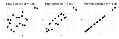
Perfect or strong Correlation ( r>0.7)
Moderate Correlation (0.5 < r < 0.7 )
Weak Correlation ( 0.3 < r < 0.5)
No Correlation ( r < 0.3()
4.4 Correlation and Regression
Correlation: Correlation measures the relationship between two variables and the strength and direction of their association. In IB studies, students might use correlation analysis to explore relationships between different data sets. For instance, in an Economics class, students might analyze the correlation between factors like inflation rates and unemployment rates to understand their relationship within an economy. In Mathematics, students might study correlation coefficients and use them to determine the strength of the linear relationship between variables.
Regression: Regression analysis helps in understanding and modeling the relationship between a dependent variable and one or more independent variables. In IB studies, regression analysis could be used to predict outcomes based on certain factors or variables. For instance, in a Biology class, students might perform linear regression to model the relationship between the concentration of a substance and the rate of a reaction. In Economics, regression analysis might be used to predict the impact of factors like government spending on GDP growth.
4.5 Probability Basics
There are several probability rules that are commonly used in probability theory. Here are a few of them:
Addition Rule: P(A or B) = P(A) + P(B) - P(A and B) This rule is used to calculate the probability of either event A or event B occurring, or both.
Multiplication Rule: P(A and B) = P(A) * P(B|A) This rule is used to calculate the probability of both event A and event B occurring.
Complement Rule: P(A') = 1 - P(A) This rule is used to calculate the probability of the complement of event A (i.e., the probability of event A not occurring).
These rules are fundamental in probability theory and are used to solve various probability problems.
4.7 D.R.V
known as Discrete Random Variables
random experiments where they are assigned a probability
Examples: a dice roll and the outcomes or a spinner and seeing the chance of an outcome in a specific section and percentage.
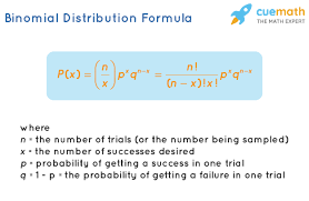
4.8 Binomial Distribution
The binomial distribution applies to events that can be described as a "success" if one outcome occurs or a "failure" if any other outcome occurs. There can be more than 2 outcomes, but it needs to be black and white in terms of success or failure.
The formula for the binomial distribution is
Where:
P(X=k) is the probability of getting exactly k successes in n independent Bernoulli trials.
n is the number of trials.
k is the number of successes.
p is the probability of success in a single trial.
Note: The binomial distribution assumes that each trial is independent and has the same probability of success.
nr)(1−p)n−rpr
4.9 Normal Distribution
The formula for the normal distribution, also known as the Gaussian distribution, is:
Where:
f(x) is the probability density function
x is the random variable
μ (mu) is the mean of the distribution
σ (sigma) is the standard deviation of the distribution
This formula describes the shape of a bell curve, with the mean at the center and the standard deviation determining the spread of the data.
5.0 X on Y Regression
another way of describing a linear regression
5.1 Conditional Independence
A concept in probability theory and statistics. It refers to the independence of two random variables given the value of a third random variable. In other words, two variables X and Y are conditionally independent given Z if the probability distribution of X and Y does not change when the value of Z is known. This can be denoted as X ⊥ Y | Z. Conditional independence is an important concept in various fields, including machine learning, graphical models, and Bayesian networks.
5.2 Normal Standardisation
Standardization refers to the process of establishing a set of guidelines or criteria to ensure consistency and uniformity in various contexts. It can be applied to different areas such as education, industry, and measurement. In education, standardization often involves the development of curriculum standards, assessment criteria, and grading systems to ensure that students are evaluated fairly and consistently. In industry, standardization aims to establish common practices, specifications, and protocols to promote interoperability and efficiency. Overall, standardization plays a crucial role in maintaining quality, reliability, and comparability in various fields.
5.3 Bayes Theorem ( HL)
Bayes' theorem is a fundamental concept in probability theory and statistics. It describes how to update the probability of a hypothesis based on new evidence. The theorem is named after Thomas Bayes, an 18th-century mathematician. In mathematical notation, Bayes' theorem can be expressed as:
P(A|B) = (P(B|A) * P(A)) / P(B)
Where:
P(A|B) is the probability of hypothesis A given evidence B.
P(B|A) is the probability of evidence B given hypothesis A.
P(A) is the prior probability of hypothesis A.
P(B) is the prior probability of evidence B.
Bayes' theorem is widely used in various fields, including machine learning, medical diagnosis, and spam filtering. It allows for the updating of beliefs or probabilities based on new information, making it a powerful tool for decision-making and inference.
5.4 C.R.V
CRV stands for Continuous Random Variable in statistics. It refers to a random variable that can take on any value within a certain range or interval. Unlike discrete random variables, which can only take on specific values, continuous random variables have an infinite number of possible values. Examples: height, weight, and time. The probability distribution of a continuous random variable is described by a probability density function (PDF) rather than a probability mass function (PMF) as in the case of discrete random variables.
The formula for a continuous random variable is the probability density function (PDF). The PDF represents the probability distribution of the random variable over a continuous range of values. It is denoted as f(x) and satisfies the following properties:
f(x) ≥ 0 for all x in the range of the random variable.
The total area under the curve of the PDF is equal to 1.
The probability of a continuous random variable falling within a specific interval [a, b] can be calculated by integrating the PDF over that interval:
P(a ≤ X ≤ b) = ∫[a, b] f(x) dx
Where X is the continuous random variable and f(x) is its PDF.
Terms
Statistics
a branch of math that goes specifically into crunching math
Mean
The average of a population
You add all of the numbers together and then dive by the amount of numbers that there are
Median
The middle
you cross the numbers out and when you get two middle numbers you add them and divide by two because this means that you are averaging them out
Mode
the value that occurs the most often
Bimodal: Two modes
Multimodal: More than 2 modes
When looking at a group of data you want to find one with the highest frequency called the modal class.
Range
the difference between the highest and lowest data values.
Probability
The likelihood that something will happen.
it can be measured numerically
Random Experiment
An experiment in which there is no way to determine the outcome beforehand
Example: is a dice game
Trial
An action in a random experiment
Example: Rolling Dice
Outcome
Possible result of a trial
Example: rolling a 2-4 on a dice
Event
Set of possible outcomes
Example: A dice is six so the outcomes of that will be 1-5, 2-4, 3-3, 4-2 and 5-1
Multiplication Rule
Mutually Exclusive Events: These are events that cannot occur simultaneously. For mutually exclusive events, the addition rule states that the probability of either one event OR another event happening is calculated by simply adding their individual probabilities.
Mathematically: P(A or B) = P(A) + P(B)
Non-Mutually Exclusive Events: These are events that can occur together. When dealing with non-mutually exclusive events, the addition rule accounts for the possibility of their overlap (the events occurring together). It's expressed as:
Mathematically: P(A or B) = P(A) + P(B) - P(A and B)
Here, P(A and B) represents the probability of both events A and B occurring simultaneously. The subtraction of P(A and B) adjusts for the double counting of the overlapping probability when summing individual probabilities.
The addition rule is fundamental in computing probabilities when considering the occurrence of events independently or jointly and helps in understanding the combined likelihood of different outcomes in various scenarios.
Multiplication Rule
the rule can apply to both independent and dependent events
two events within one sample space
Dependent Events
P(A ∩ B) = P(B). P(A|B)
Independent Events
P(A ∩ B) = P(A). P(B)
Frequency distributions
a list of each category and the number of occurrences for each of the categories of data
Standard Deviation
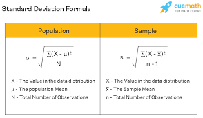
measures the deviation between scores and the mean.
It’s the square root of the variance
A sort of average of differences between the values and the mean.
The symbol for Standard Deviation is σ
It is normally distributed
Deviation
The difference between the data values of X and the mean.
Binomial Distribution
It applies to the following:
When a distribution is discrete
In a fixed number of trials
When there is a success and a failure
When the probability of success is the same for all of the trials which is when the trials are independent
Random Variables
Random variables are a key concept in probability and statistics, representing numerical outcomes of random phenomena. They are used to quantify uncertain events in a mathematical framework.
A random variable, often denoted by a capital letter such as X, Y, or Z, assigns a numerical value to each outcome of a random experiment. There are two types of random variables: discrete and continuous.
Discrete Random Variables
a random variable that has either a finite or countable number of values.
The values can be plotted on a number line with space between each point.
Continuous Random Variables
A variable that has infinitely many values.
The values can be plotted on a line in an uninterrupted fashion.
Binomial Distribution and Probability
Chi-Square
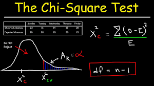
Goodness of Fit
a statistical test that tries to determine whether a set of observed values match those expected under the applicable model.
Cumulative Frequency Distribution
The graphs can be used to estimate the median and to find other properties of the data.
A distribution that displays the aggregate frequency of a category can also be known as discrete data. It displays the total number of observations which are less than or equal to the categories.
For the continuous data: they observe the total number of observations that are less than or equal to the upper class limit of a class.
Cumulative Relative Frequency Distribution
A distribution that displays a proportion or a percentage of observations that are less than or equal to the categories of the discrete data. This can also be the proportion or percentage of observations that are less than or equal to the upper-class limits of the continuous data.
Hypothesis Testing
An assumption about a population parameter such as a mean or a proportion. This assumption may or may not be true
A hypothetical estimate of what an outcome may be
If one hypothesis is true then the other one must be false
Stating either the null or the alternative hypothesis depends on the nature of the test as well as the motivation of the person who is conducting the specific test
Alternative Hypothesis ( H0)
new drug on a different effect on average compared to that of a new and current drug or that the new drug is better on average than the current drug
opposite of the null hypothesis
it is believed to be true if the null hypothesis is found to be false
never use the equal sign
used in the research hypothesis as well as the claim that the researchers wish to support
Null Hypothesis(H1)
always use an equal sign
Can be used with standard deviation
tested using the sample data
represents the status quo
belief that the population parameter is greater than or equal to a specific value.
beloved to be true unless there is an overwhelming evidence
might be that the new drug is no better, on average than the current drug.
Logic of Hypothesis
Reject
Fail to reject
Types of Testing
Left Tailed Test
population mean is less than a specific value K
Right Tailed Test
population mean is greater than a specific value K
One tail test
left or right-tailed
Two-Tailed Test
two critical values
reject or the other one
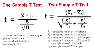
T-test
Z- Score

R-value
Different Types of Graphs
Vocabulary For Graphs
Outlier
a data point whose values is significantly greater than or less than the other values
Cluster
an isolated group of points
Gap
a large space between the data points
Histograms
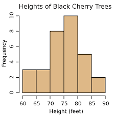
Definition: a drawing of each class using rectangles. The height of each rectangle is the frequency or relative frequency of the class. The width of the rectangles are all the same and the rectangles also do not touch each other.
contain a commonality or what they are testing which is the height in feet of how tall the Black Cherry Trees grow
contain the frequency which is how often something happens which is in this case how often the specific Black Cherries grow on trees
Stem and Leaf Plots
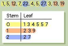
Stem: the digits on the left side of the rightmost digits of the raw data
Leaf: the rightmost digit in the plot
it is similar to a dot plot but the number that the line is vertical and there are numbers used instead of X’s
A representation of graphical quantitative data in which the data itself is used to create a certain graph. The raw data gets retrieved from the graph.
Box and Whisker Plots also known as a Box Plot

A type of graph that shows the dispersion of data
a quick and simple way of organizing numerical data.
Normally used when there is only one group of data with less than 50 values
Five number summary
Upper Quartile(Q3):
Lower Quartile(Q1):
Interquartile Range (IQR): The difference between upper and lower quartiles Q3-Q1.
Pareto Chart
a bar graph whose bars are drawn in decreasing order of frequency or relative frequency
Pie Chart
a circle divided into sectors where each of the sectors represents a category of a certain data. The area of each of the sectors is proportional to the frequency of each of the categories.
Dot Plot
they are drawn by placing each of the observations horizontally in the increasing order in which a dot is placed above the observation every time that it is observed
Time Series Plot
they are obtained by plotting time in which a variable is measured on a horizontal axis and where the corresponding value of the variable is located on the vertical axis. The line segments
Ogive
a graph that represents the cumulative or cumulative relative frequency of a class. They are constructed by plotting points which
Degree of Confidence or the Confidence level
The confidence interval actually does ensure that the population parameter
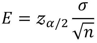
Margin of Error
 dC
dC
Population Proportion
The population proportion refers to the proportion or percentage of individuals in a population that exhibits a certain characteristic or have a specific attribute of interest. It represents the ratio of the number of individuals possessing a particular trait to the total population size.
For instance, imagine a population of 1000 people, and out of these, 300 individuals have brown hair. The population proportion of individuals with brown hair would be calculated by dividing the number of individuals with brown hair by the total population size:
Population Proportion of Brown-Haired Individuals = Number of Brown-Haired Individuals / Total Population Size Population Proportion of Brown-Haired Individuals = 300 / 1000 = 0.3 or 30%
in statistical terms, if you were to take multiple random samples from this population and calculate the proportion of brown-haired individuals in each sample, the average of these sample proportions would typically converge toward the population proportion as the sample size increases, following the principles of the law of large numbers and the central limit theorem.
Estimating population proportions and understanding their variability through statistical inference is important in various fields such as public health, sociology, market research, and more. Techniques such as confidence intervals and hypothesis testing are used to make inferences about population proportions based on sample data.