Analysis of Two Conditions

The analysis of two conditions includes the following:

1. Descriptive statistics, such as means or medians, and standard deviations; confidence intervals around the mean of both groups separately, where this is appropriate; graphical illustrations such as box and whisker plots and error bars.

2. Effect size: this is a measure of the degree to which differences in a dependent variable are attributed to the independent variable.

3. Confidence limits around the difference between the means.

4. Inferential tests: t-tests discover how likely it is that the difference between the conditions could be attributable to sampling error, assuming the null hypothesis to be true

7.1.1 Analysis of Differences between Two Independent Groups

Example:

Twenty-four people were involved in an experiment to determine whether background noise (music, slamming of doors, people making coffee, etc.) affects short-term memory (recall of words). Half of the sample were randomly allocated to the NOISE condition, and half to the NO NOISE condition. The participants in the NOISE condition tried to memorize a list of 20 words in two minutes, while listening to pre-recorded noise through earphones. The other participants wore earphones but heard no noise as they attempted to memorize the words. Immediately after this, they were tested to see how many words they recalled.

7.1.2 Descriptive Statistics for Two-Group Design

• The first thing to do is to obtain descriptive statistics. You can then gain insight into the data by looking at graphical illustrations, such as box and whisker plots and/or histograms.

7.1.3 Confidence Limits Around the Mean

• The means you have obtained, for your sample, are point estimates. These sample means are the best estimates of the population means.

• Our estimate could be slightly different from the real population mean difference: thus it would be better, instead of giving a point estimate, to give a range. This is more realistic than giving a point estimate.

• The interval is bounded by a lower limit and an upper limit. These are called confidence limits, and the interval that the limits enclose is called the confidence interval. The confidence limits let you know how confident you are that the population mean is within a certain interval: that is, it s an interval estimate for the population (not jut your sample).

• Why confidence limits are important

  • When we carry out experiments or studies, we want to be able to generalize from our particular sample to the population.

7.1.4 Confidence Intervals between NOISE and NO NOISE Conditions

• For the noise condition, we estimate (with 95% confidence) that the population mean is within the range (interval) of 5.7 and 8.8.

7.1.5 Measure of Effect

We can also take one (sample) mean from the other, to see how much they differ:

7.3 - 13.8 = -6.5

This score on its own, however, tells us very little. If we converted this score to a standardized score, it would be much more useful. The raw score (the original score) is converted into a z-score. The z-score is a standardized score, giving a measure of effect which everyone can easily understand. This measure of effect is called d; d measures the extent to which the two means differ, in terms of standard deviations. This is how we calculate it:

d = (x1 - x2)/ (mean SD)

This means that we take one mean away from the other (it does not matter which is which – ignore the sign) and divide it by the mean standard deviation.

Step 1: find mean sample SD

(SD of condition 1 + SD of condition 2)/ 2 = (2.5 + 2.8)/ 2 = 2.65

Step 2: find d

(x1 - x2)/ (mean SD) = (7.3 - 13.8)/ 2.65 = 6.5 / 2.65 = 2.45

In this case, our means differ by 2.45 standard deviations. This is a very large effect size, an effect size not often found in psychological research

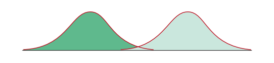
7.1.6 The Size of the Effect

• When there is little difference between our groups, the scores will overlap substantially.

• If there is a large difference between the two groups, then the distributions will be further apart.

7.1.7 Inferential Statistics: The t-test

• The t-test is used when we have two conditions. The t-test assesses whether there is a statistically significant difference between the means of the two conditions.

• Independent t-test: is used when the participants perform in only one of two conditions: that is, an independent, between-participants or unrelated design.

• Related or Paired t-test: is used when the participants perform in both conditions: that is, a related, within-participants or repeated measures design.

• The t-test was devised by William Gossett in 1908. Gossett worked for Guinness, whose scientists were not allowed to publish results of their scientific work, so Gossett published results using his new test under the name of Student, which is why you will see it referred to in statistical books as Student’s t.

• If in practice, we obtain a t-value that is found in one of the tails, then we conclude that it is unlikely to have arisen purely by sampling error.

• Each obtained t-value comes with an exact associated probability level.

• If, for instance, our obtained t has an associated probability level of 0.03, we can say that, assuming the null hypothesis to be true, a t-value such as the one we obtained in our experiment would be likely to have arisen in only 3 occasions out of 100. Therefore, we conclude that there is a difference between conditions that cannot be explained by sampling error.

7.1.8 Output for Independent t-test

Means of the two conditions and the difference between them

• What you want to know is whether the difference between the two means is large enough to be important (not only ‘statistically significant’, which tells you the likelihood of your test statistic being obtained, given that the null hypothesis is true).

Confidence Intervals

• SPSS, using the t-test procedure, gives you confidence limits for the difference between the means.2 The difference between means, for your sample, is a point estimate. This sample mean difference is the best estimate of the population mean difference. If, however, we repeated the experiment many times, we would find that the mean difference varied from experiment to experiment. The best estimate of the population mean would then be the mean of all these mean differences. It is obviously better to give an interval estimate, as explained before. Confidence limits let you know how confident you are that the population mean difference is within a certain interval. That is, it is an interval estimate for the population (not just for your sample)

t-value

• The higher the t-value, the more likely it is that the difference between groups is not the result of sampling error. A negative value is just as important as a positive value. The positive/negative direction depends on how you have coded the groups.

p-value

• This is the probability of your obtained t-value having arisen by sampling variation, or error, given that the null hypothesis is true. This means that your obtained t is under an area of the curve that is uncommon – by chance, you would not expect your obtained t-value to fall in this area. The p-value shows you the likelihood of this arising by sampling error.

Degrees of Freedom (DF)

• For most purposes and tests (but not all), degrees of freedom roughly equate to sample size. For a related t-test, DF are always 1 less than the number of participants. For an independent t-test, DF are (n1 - 1)+(n2 - 1)(cubed) so for a sample size of 20 (10 participants in each group), DF = 18 (i.e. 9 + 9). For a within-participants design with sample size of 20, DF = 19. DF should always be reported in your laboratory reports or projects, along with the t-value, p-value and confidence limits for the difference between means. Degrees of freedom are usually reported in brackets, as follows: t (87) = 0.78 This means that the t-value was 0.78, and the degrees of freedom 87.

Standard Deviations

• This gives you the standard deviation for your samples.

Standard Error of the Mean (SEM)

• This is used in the construction of confidence intervals.

7.1.9 Assumptions to be Met in using t-tests

• The t-test is a parametric test, which means that certain conditions about the distribution of the data need to be in force: that is, data should be drawn from a normally distributed population of scores.

• The t-test is based on the normal curve of distribution. Thus, we assume that the scores of our groups, or conditions, are each normally distributed. The larger the sample size, the more likely you are to have a normal distribution. As long as your data are reasonably normally distributed, you do not need to worry, but if they are severely skewed, you need to use a non-parametric test.

• Remember that in using the t-test we compare a difference in means, and if our data are skewed, the mean may not be the best measure of central tendency.

7.1.11 Related t-test

• The related t-test is also known as the paired t-test; these terms are interchangeable.

• The related t-test is used when the same participants perform under both conditions.

• The related t-test is more sensitive than the independent t-test. This is because each participant performs both conditions, and so each participant can be tested against him- or herself. So the formula for the related t-test takes into account the fact that we are using the same participants.

• Related t-test gives a result with a higher associated probability value -- this is because the comparison of participants with themselves gives rise to a reduced within-participants variance, leading to a larger value of t.