Chapter 3: Differentiation
A. Definition of Derivative
At any x in the domain of the function y = f(x), the derivative is defined as
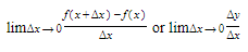
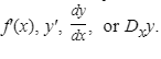
The function is said to be differentiable at every x for which this limit exists, and its derivative may be denoted by
Frequently ∆x is replaced by h or some other symbol.
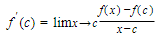
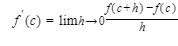
The derivative of y = f(x) at x = a, denoted by f′(a) or y′(a), may be defined as follows:
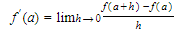
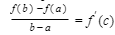
The fraction
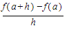
is called the difference quotient for f at a and represents the average rate of change of f from a to a + h.
Geometrically, it is the slope of the secant PQ to the curve y = f(x) through the points P(a, f(a)) and Q(a + h, f(a + h)).
The limit, f′(a), of the difference quotient is the (instantaneous) rate of change of f at point a.
Geometrically, the derivative f′(a) is the limit of the slope of secant PQ as Q approaches P—that is, as h approaches zero.
This limit is the slope of the curve at P.
The tangent to the curve at P is the line through P with this slope.
PQ is the secant line through (a, f(a)) and (a + h, f(a + h)).
The average rate of change from a to a + h equals RQ/PR, which is the slope of secant PQ.
PT is the tangent to the curve at P.
As h approaches zero, point Q approaches point P along the curve, PQ approaches PT, and the slope of PQ approaches the slope of PT, which equals f′(a).
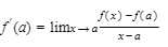
If we replace (a + h) by x, in (2) above, so that h = x − a, we get the equivalent expression
The second derivative, denoted by
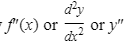
is the (first) derivative of f′(x).
Also, f″(a) is the second derivative of f(x) at x = a.
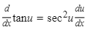
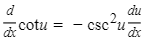
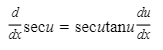
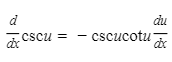
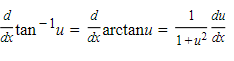
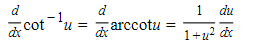
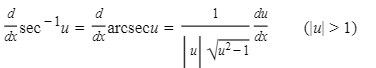
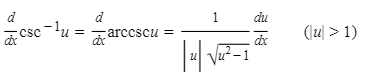
B. Formulas
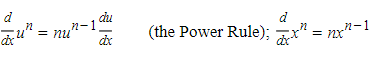
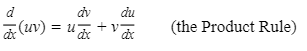
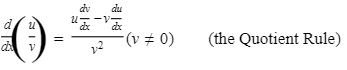
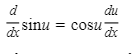
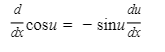
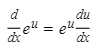
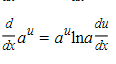
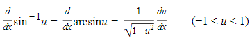
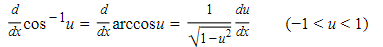
The formulas in this section for finding derivatives are so important that familiarity with them is essential. If a and n are constants and u and v are differentiable functions of x, then:
2.  3.
3.  4.
4. 
5.  6.
6. 
7.  8.
8.  9.
9.  10.
10.  11.
11.  12.
12.  13.
13.  14.
14.  15.
15.  16.
16.  17.
17.  18.
18.  19.
19.  20.
20.  21.
21. 
C. The Chain Rule; The Derivative of Composite Function
Formula 3 says that: 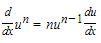
This formula is an application of the Chain Rule.
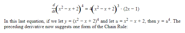
For example, if we use formula 3 to find the derivative of (x2 − x + 2)^4, we get:
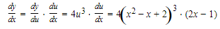
Now suppose we think of y as the composite function f(g(x)), where y = f(u) and u = g(x) are differentiable functions. Then
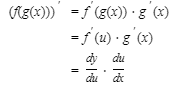
The Chain Rule tells us how to differentiate the composite function:
“Find the derivative of the ‘outside’ function first, then multiply by the derivative of the ‘inside’ one.”
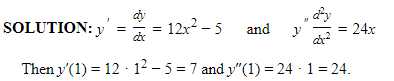
Example:
If y = 4x3 − 5x + 7, find y′(1) and y″(1).
SOLUTION:
D. Differentiability and Continuity
If a function f has a derivative at x = c, then f is continuous at x = c.
This statement is an immediate consequence of the definition of the derivative of f′(c) in the form
If f′(c) exists, then it follows that limx→cf(x)=f(c), which guarantees that f is continuous at x = c.
If f is differentiable at c, its graph cannot have a hole or jump at c, nor can x = c be a vertical asymptote of the graph. The tangent to the graph of f cannot be vertical at x = c; there cannot be a corner or cusp at x = c.
Each of the “prohibitions” in the preceding paragraph (each “cannot”) tells how a function may fail to have a derivative at c.
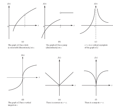
The graph in (e) is for the absolute function, f(x) = |x|. Since f′(x) = −1 for all negative x but f′(x) = +1 for all positive x, f′(0) does not exist.
We may conclude from the preceding discussion that, although differentiability implies continuity, the converse is false.
The functions in (d), (e), and (f) in are all continuous at x = 0, but not one of them is differentiable at the origin.
E. Estimating a Derivative
E1. Numerically
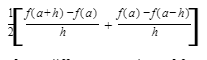
From a Symmetric Difference Quotient
We can also estimate f′(a) numerically using the symmetric difference quotient, which is defined as follows:
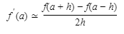
Note that the symmetric difference quotient is equal to
 Example:

SOLUTION:
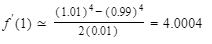 The exact value of f′(1), of course, is 4.
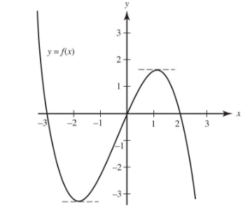
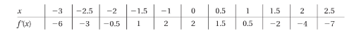
E2. Graphically
If we have the graph of a function f(x), we can use it to graph f′(x).
We accomplish this by estimating the slope of the graph of f(x) at enough points to assure a smooth curve for f′(x). In the figure below, we see the graph of y = f(x).
Below it is a table of the approximate slopes estimated from the graph.
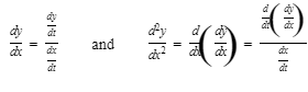
F. Derivatives of Parametrically Defined Functions
If x = f(t) and y = g(t) are differentiable functions of t, then
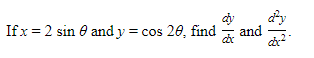
Example:
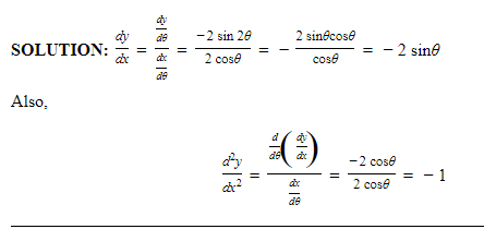
Solution:
G. Implicit Differentiation
When a functional relationship between x and y is defined by an equation of the form F(x,y) = 0, we say that the equation defines y implicitly as a function of x.
Implicit differentiation is the technique we use to find a derivative when y is not defined explicitly in terms of x but is differentiable.
Example:
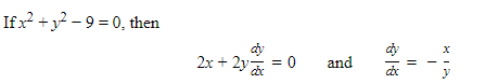
Note that the derivative above holds for every point on the circle, and exists for all y different from 0 (where the tangents to the circle are vertical)
H. Derivative of the Inverse of a Function
The graphs of inverse functions are the reflections of each other in the line y = x, and that at corresponding points their x- and y- coordinates are interchanged.
The figure below shows a function f passing through point (a, b) and the line tangent to f at that point.
The slope of the curve there, f′(a), is represented by the ratio of the legs of the triangle, dy/dx. When this figure is reflected across the line y = x, we obtain the graph of f−1, passing through point (b,a), with the horizontal and vertical sides of the slope triangle interchanged.
Note that the slope of the line tangent to the graph of f−1 at x = b is represented by dx/dy, the reciprocal of the slope of f at x = a.
We have, therefore
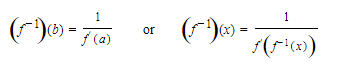
The derivative of the inverse of a function at a point is the reciprocal of the derivative of the function at the corresponding point.
Example:
If f(3) = 8 and f′(3) = 5, what do we know about f−1?
SOLUTION:
Since f passes through the point (3,8), f−1 must pass through the point (8,3). Furthermore, since the graph of f has slope 5 at (3,8), the graph of f−1 must have slope 1/5 at (8,3).
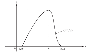
I. The Mean Value Theorem
If the function f(x) is continuous at each point on the closed interval a ⩽ x ⩽ b and has a derivative at each point on the open interval a < x < b, then there is at least one number c, a < c < b, such that
This important theorem, which relates average rate of change and instantaneous rate of change.
For the function sketched in the figure there are two numbers, c1 and c2, between a and b where the slope of the curve equals the slope of the chord PQ (i.e., where the tangent to the curve is parallel to the secant line).
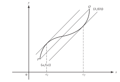
We will often refer to the Mean Value Theorem by its initials, MVT.
If, in addition to the hypotheses of the MVT, it is given that f(a) = f(b) = k, then there is a number, c, between a and b such that f′(c) = 0. This special case of the MVT is called Rolle’s Theorem, for k = 0.
Example:
You left home one morning and drove to a cousin’s house 300 miles away, arriving 6 hours later. What does the Mean Value Theorem say about your speed along the way?
SOLUTION:
Your journey was continuous, with an average speed (the average rate of change of distance traveled) given by
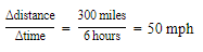
Furthermore, the derivative (your instantaneous speed) existed everywhere along your trip. The MVT, then, guarantees that at least at one point your instantaneous speed was equal to your average speed for the entire 6-hour interval. Hence, your car’s speedometer must have read exactly 50 mph at least once on your way to your cousin’s house.
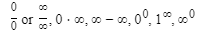
J. Indeterminate and L’hospital’s Rule
Limits of the following forms are called indeterminate:
To find the limit of an indeterminate form of the type 0/0 or ∞/∞, we apply L’Hospital’s Rule, which involves taking derivatives of the functions in the numerator and denominator.
In the following, a is a finite number. The rule has several parts:
a. 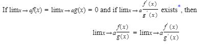
b. If limx→af(x)=limx→ag(x)=∞, the same consequences follow as in case (a). The rules in (a) and (b) both hold for one-sided limits.
c. 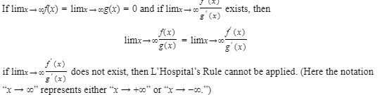
d. If limx→∞f(x)=limx→∞g(x)=∞, the same consequences follow as in case (c).
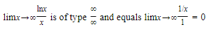
Example:
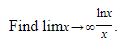
SOLUTION:
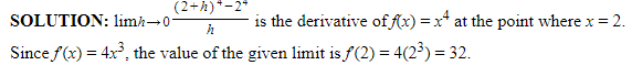
K. Recognizing a Given Limit as a Derivative
It is often extremely useful to evaluate a limit by recognizing that it is merely an expression for the definition of the derivative of a specific function (often at a specific point).
The relevant definition is the limit of the difference quotient:
Example:
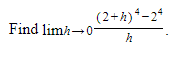
SOLUTION: