


AP Microeconomics Ultimate Guide
Complete guide for all information relating to the basics of economic concepts
Unit 1 - Basic Economic Concepts
1.1 - Scarcity
Economics in general is a study of how an entity, whether it be an individual or an organization, manages and allocates its resources in the most efficient way possible. The need to allocate and organize resources is derived from the basic concept of scarcity which exists. This doesn’t just apply to money management, politics, or the stock market
The economic problem states however that our needs our unlimited and as mentioned earlier, the resources available are scarce.
In the realm of economics, all resources around us are considered to be limited; even the most basic things which exist around us like air or water
Scarcity : unlimited wants, limited resources (example : land). Where society does not enough resources to produce the goods and services which everybody needs. As a consumer, we must make choice as to how to allocate resources properly.
Microeconomics Vs. Macroeconomics
Microeconomics: filters our scope to individuals in an economy while keeping the overall economy in mind. Focuses is directed at the roles households and firms play and how their decision-making and allocation of resources impact the overall economy.
Macroeconomics: we consider the big picture- the nation’s economy as a whole. E.g. would changes to the money supply have an effect on country A’s imports and export? This branch studies the behaviour and performance of the entire economy
Factors of production
These are resources that are scarce, can be broken down into four categories:
Land: natural resources and raw material. Ex: water, oil, minerals and such.
Labor: physical labor, skills, and effort devoted into a task where workers are paid.
Capital: is usually referred to as the liquid asset, or monetary value
Physical capital: tools and equipment used to produce a good or service
Human capital: education and training an individual has that is used in the production of a good or service
Entrepreneurship: the ability of an individual to coordinate the other categories of resources to produce a good or service
Opportunity Costs and Trade-offs
Trade-offs: The alternative choice which must be given up in order to make a decision. The goods and services which you do not choose are the trade-offs.
Opportunity costs: This is the cost we forgo or sacrifice, to opt for another choice. The next best alternative if your first choice is unavailable.
Positive vs Normative Economics
The study of Economics can be broken down into 2 more ways,
Positive Economics: this approach to economics is based on facts and figures.
Theories to understand behavior are proved via a full procedure of hypothesis and testing. E.g. Increase in income for family A, increases their spending but not by the same amount as the change in income
Normative Economics: this approach to economics is based on assumptions.
Economic behaviors are first analyzed and then evaluated based on the researcher’s opinion. E.g. Refurbishment schemes can cause a decrease in the prices of second-hand phones
Both these approaches are crucial for the study of economics since economic theories are the core of our study, and theories require a hypothesis that is shaped based on what an individual feels or thinks
1.2 - Resource Allocation and Economic Systems
There are 3 big economic questions, what, how, and for whom?
What goods and services will be produced? The economy has to decide what goods and services the society needs in order to properly allocate resources.
How will goods and services be produced? This deals with how businesses will go about producing these goods and services.
For whom will the goods and services be produced? This question decides who will be able to consume these goods and services, to where these resources where will be allocated.
Types of Economic Systems
Centrally-Planned (Command) Economic System:
Here, the government makes all the economic decisions and answers the three questions on its own. They set the prices for goods and services, as well as set wage rates. However, they do not respond to consumer wants, and innovation is discouraged.
Market Economic System:
Economic changes are guided by the changes in price which occur as individuals and sellers interact in the market. There is a lot of competition and a variety of goods and services. However, there will be a wealth disparity in the market.
Mixed Economic System:
A system which has characteristics of both central system and market economic system. There are private property rights which are protected, however, the government is able to intervene in order to meet societal aims.
1.3 - Production Possibilities Curve
Represents the best possible combinations of goods, given a fixed amount of resources. In the graph, we can note than resources and technology is mixed, and only two goods can be made.
Illustrates the trade-offs that faces an economy, compares only two goods
If the PPC is linear, it has a constant opportunity cost, if it is curved, it has increasing opportunity costs
Economic growth : a sustained rise in aggregate output and an increase in standard of living (causes are developments in technology, or an increase in resources)
Productive efficiency : lowest cost possible on the PPC
Allocative efficiency : the economy allocates resources so consumers are well off as possible, producing what is demanded
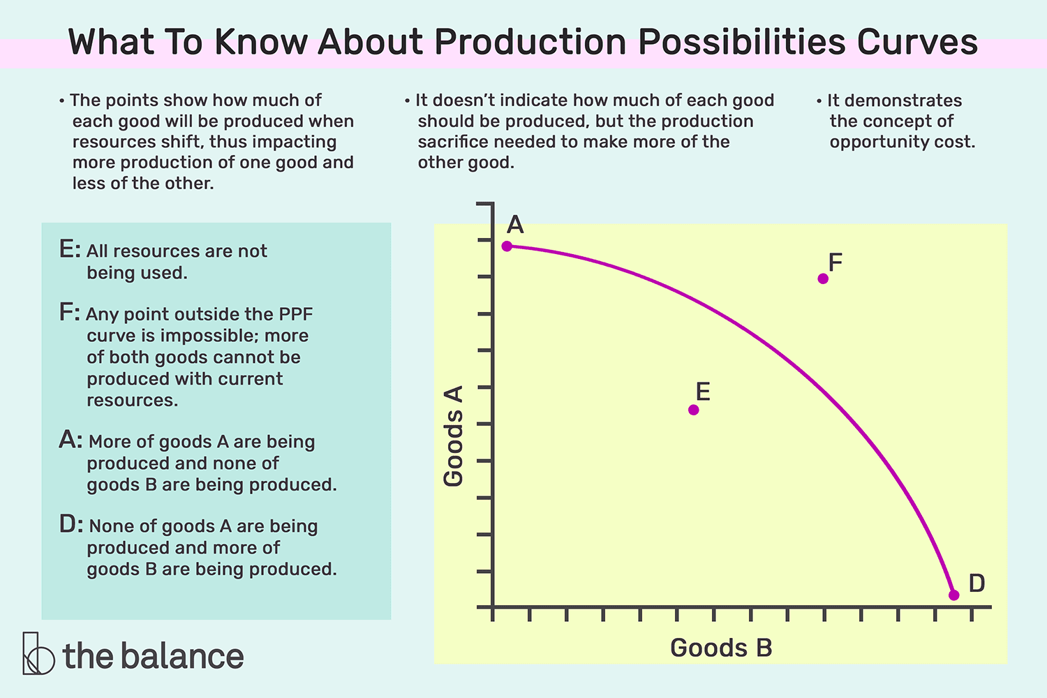
Constant opportunity cost
Occurs when OC stays the same as the production of a good increases.
Increasing opportunity cost
When one good is produced more, you give up more of another good.
Determinants of PPC
The curve can shift upwards or downwards respectively due to certain factors:
Changes in the amount of resources in the economy:
This could be due to changes in the labor force because of population changes, acquirement of new territories (e.g. for farming, mining), or destruction of territories due to weather conditions, etc.
Changes in technology and productivity:
This could be due to government schemes to help farmers for instance or could be due to the usage of inefficient production techniques, etc
Trade:
This is dependent on new resources being discovered or improve production techniques.
1.4 - Comparative Advantage and Trade
Absolute Advantage: Occurs when a firm as the ability to produce a specific amount of goods or services in comparison to the others.
Comparative Advantage: The ability of a firm to produce a good or service at the lowest possible cost
Terms of Trade: people split up the work, and provide each other with a good in return for another. It is also the rate at which one good can be exchanged for another (if the price of a good obtained from trade is less than the opportunity cost of producing it, trade is beneficial)
Capital goods: goods that make consumer goods (ex. machinery)
Consumer goods : goods that are consumed (ex. food)
1.5 - Cost-Benefit Analysis
Implicit costs: monetary or non-monetary opportunity costs in terms of making a choice.
Explicit costs: traditional out of pocket costs which are associated with choosing one course of action.
1.6 - Marginal Analysis and Consumer Choice
Utility: the measure of personal satisfaction (util is a unit of utility)
Marginal utility: the change in total utility by consumer one additional unit of that good/service
Principle of diminishing marginal utility : additional units of a good/service add less total utility than the previous units do
Marginal utility per dollar : MUgood/Pgood (marginal utility of one unit of the good / price of one unit of the good)
Optimal consumption rule : to maximize utility, marginal utility per dollar spend on each good = service in consumption bundle, MUc/Pc = MUt/Pt
Unit 2 - Supply and Demand
All the basics of Supply and Demand which are the foundation of the majority of concepts moving forward.
2.1 - Demand
Demand: the quantity which a consumer/buyer are willing and able to buy at different prices
Movement on the graph: downward sloping
Demand slopes down on the graph due to:
Income effect
Substitution effect
law of diminishing marginal utility
Law of Demand: As price increases, demand decreases, and as price decreases, demand increases
Determinants of demand:
Taste and preferences, related goods, income, buyers, expectation of failure
Substitutes : good/service that can be used in place of another, when price of one increases, consumers will buy more of the other (ex. coffee and tea)
Substitution effect: as the price of a good increases, consumers substitute the good with another that is cheaper
Complements : goods/services that are consumed together (ex. hamburgers and buns)
Income effect: as income increases, people will buy more of normal goods, and less of inferior goods
Normal good : increase in demand when consumer’s income increases (ex. oreos)
Inferior good : increase in demand when consumer’s income decreases (ex. off brand oreos)
Diminishing marginal utility: As more units of a product are consumed, the satisfaction/utility it provides tends to decline
Apple users would purchase at maximum, a limited phones-they wouldn’t purchase a new iPhone every month since that extra phone would offer them no utility or not as much
2.2 - Supply
Supply: different quantities of goods/services which sellers are willing and able to produce at a given price
Law of supply: as price increases, quantity supplied also increases, this is a direct relation.
The market supply shows the quantity a supplier is willing and able to offer at various prices at a given time
Reasons for the Law of Supply
Rising prices give greater opportunities to suppliers to earn a profit
With every additional unit, suppliers face an increase in the marginal cost of production
Charging higher prices provides them with the easiest way to cover the cost
The vice versa is also true; lower prices wouldn’t provide the incentive to motivate the supplier and thus reduces the quantity of product
The supply curve shifts upward, and the movement along the supply curve indicates a change in price.
Shifters of supply :
Resource costs and availability
The cost of production (land, labor, capital) has an inverse impact on the supply
When the cost of these increases, the supplier decides to produce less of the products since he is unable to afford the production cost
Other goods and services
Suppliers who produce more than one product (profit-maximizing firms) have an easier time switching to the production of another product if issues do arise in prices
E.g. A farmer has land where he is able to produce corn and earn a profit
If his land is capable to produce wheat as well, in case the price of wheat increases to that of corn, he would switch to wheat production to earn better
The supply curve in this situation for wheat would shift outwards(more supply) and vice versa for corn(reduced supply)
Technology
Newer technology causes the cost of production to decline and helps improve the efficiency of the supplier
This allows the supplier to produce more, shifting the supply curve outwards(toward right)
E.g. machines on the production line help reduce unit costs due to which more products are affordable by the supplier
Taxes and Subsidies
Taxes are added up to the unit cost of production, thus making it more expensive
Due to this, heavily taxed products are produced in less quantity by suppliers(supply curve shifts towards left)
Subsidies are the opposite of taxes and help reduce price per unit
This allows suppliers to produce more of the product(supply curve shifts towards the right)
Expectation
If suppliers expect prices to increase in the future, they would hold back supply for the current time with the future goal of earning more profit later (and vice versa)
Number of sellers
As the number of sellers increases in the market, the supply automatically increases
This allows consumers more choices at a lower price due to an increase in competition
2.3 - Price Elasticity of Demand
Equation : %∆Qd/%∆P
0 = perfectly elastic, <1 = inelastic, =1 unit elastic, >1 = elastic
Midpoint formula : Qd2-Qd1/(Q2d+Qd1)/2 , replace with Qd with price for price
Inelastic demand : TR correlates direct with price
Elastic demand = TR correlates inversely with price
Elasticity: how much the Q is affected by P.
Elastic demand means that the goods are subject to be affected by a change in price.
Inelastic demand means that goods are not subject to be affected by a change in price.
Characteristics of Elastic Demand:
Flat, quantity is sensitive to price change, substitutes, luxury items, large portion of income, not needed immediately. Is equal to >1.
Characteristics of Inelastic Demand:
Steep, few substitutes, required now, small portion of income, is equal to <1
Shapes of elasticity/inelasticity
Perfectly elastic: infinity
Relatively elastic: >1
Unit elastic: 1
Relatively inelastic: <1
Perfectly inelastic: 0
2.4 - Price Elasticity of Supply
PES: measures how sensitive are sellers to price changes on goods
Equation : %∆Qs/%∆P
0 = perfectly elastic, <1 = inelastic, =1 unit elastic, >1 = elastic
Inelastic : unable to respond to price change
Elastic : short run
Extremely elastic : long run
Characteristics of inelastic Supply:
Difficult production, high costs, hard to change to alternative, high barriers to entry, <1
Characteristics of Elastic Supply:
Easy production, low cost, easy to switch to, low barriers to entry, >1
2.5 - Other Elasticities
Cross price elasticity of demand : %∆Qd of Good A/%∆P of good B
Negative = compliments (inferior good), positive = substitutes (normal good)
Income elasticity of demand : %∆Qd/%∆income
1 = income elastic, <1 = income inelastic, negative = inferior, positive = normal
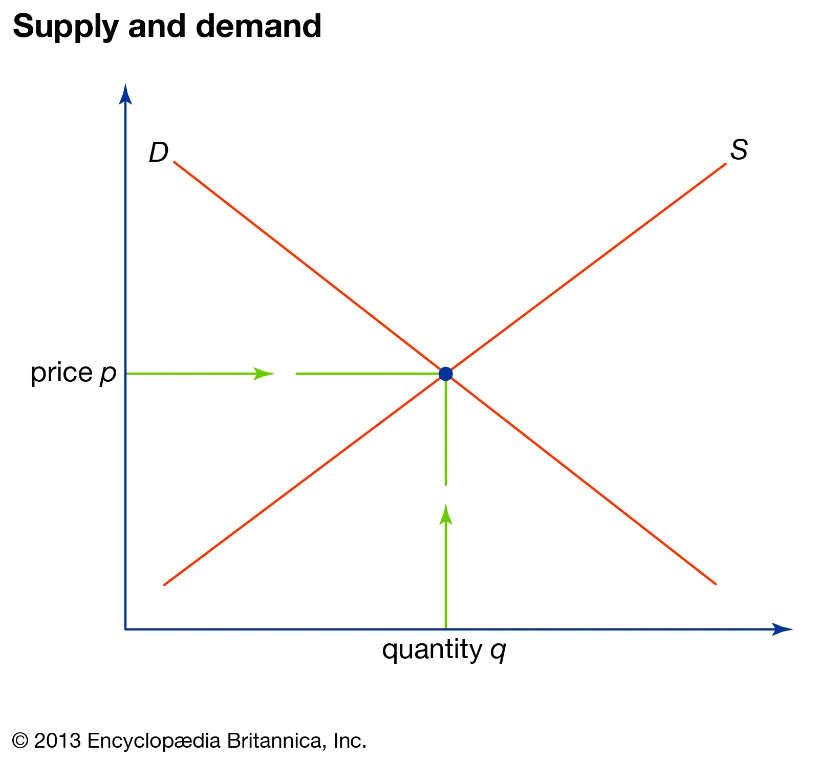
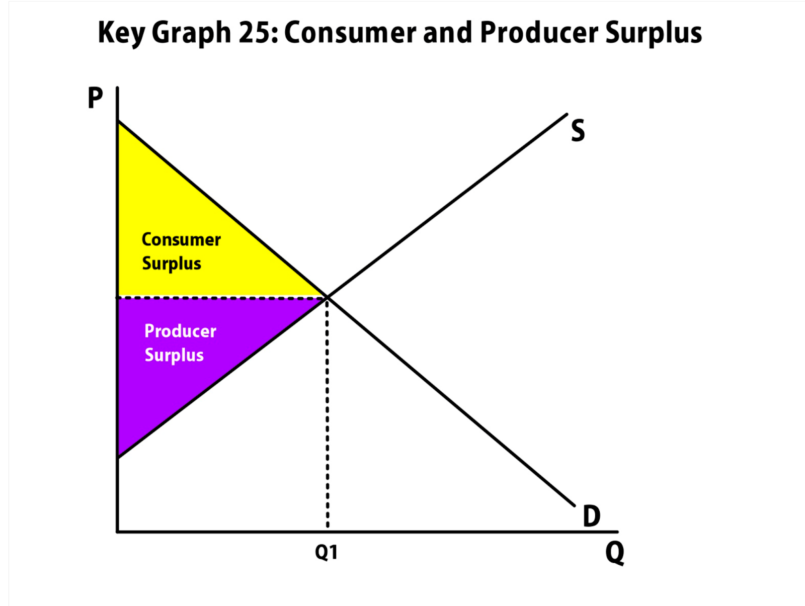
2.6 - Market Equilibrium, Consumer and Producer Surplus
Equilibrium : occurs when no one is better off doing something else
Equilibrium = Qs=Qd
Price below the equilibrium is shortage
Consumer surplus : price consumers are willing to pay - actual price
Producer surplus : actual price -price the producer is willing to sell for
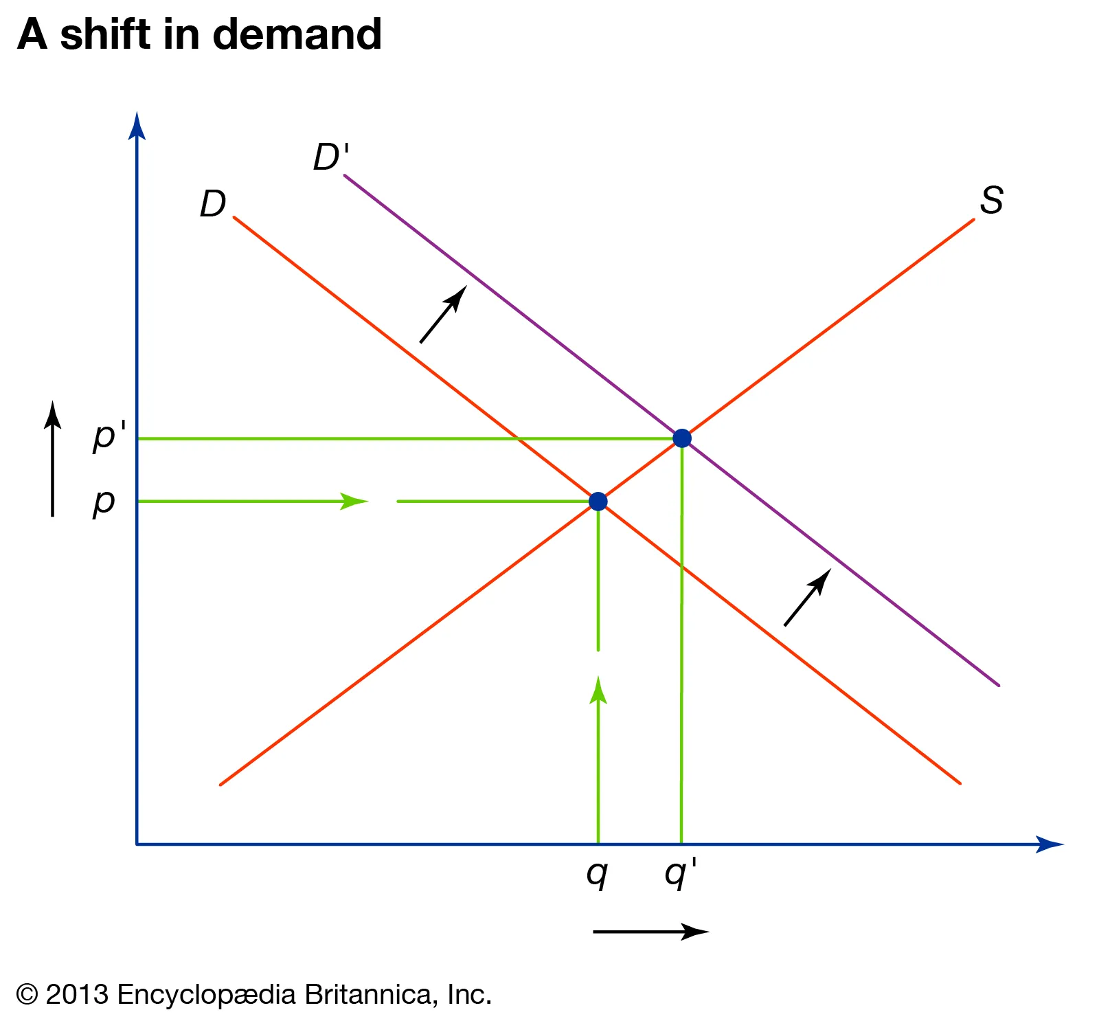
Demand increase : price and quantity increase
Demand decrease : price and quantity decrease
Supply increase : price decreases, quantity increases
Supply decrease : price increases, quantity decreases
Double shift : either price or quantity will be unknown. This rule states that when there is a simultaneous shift in both demand and supply, either price or quantity would stay indeterminate
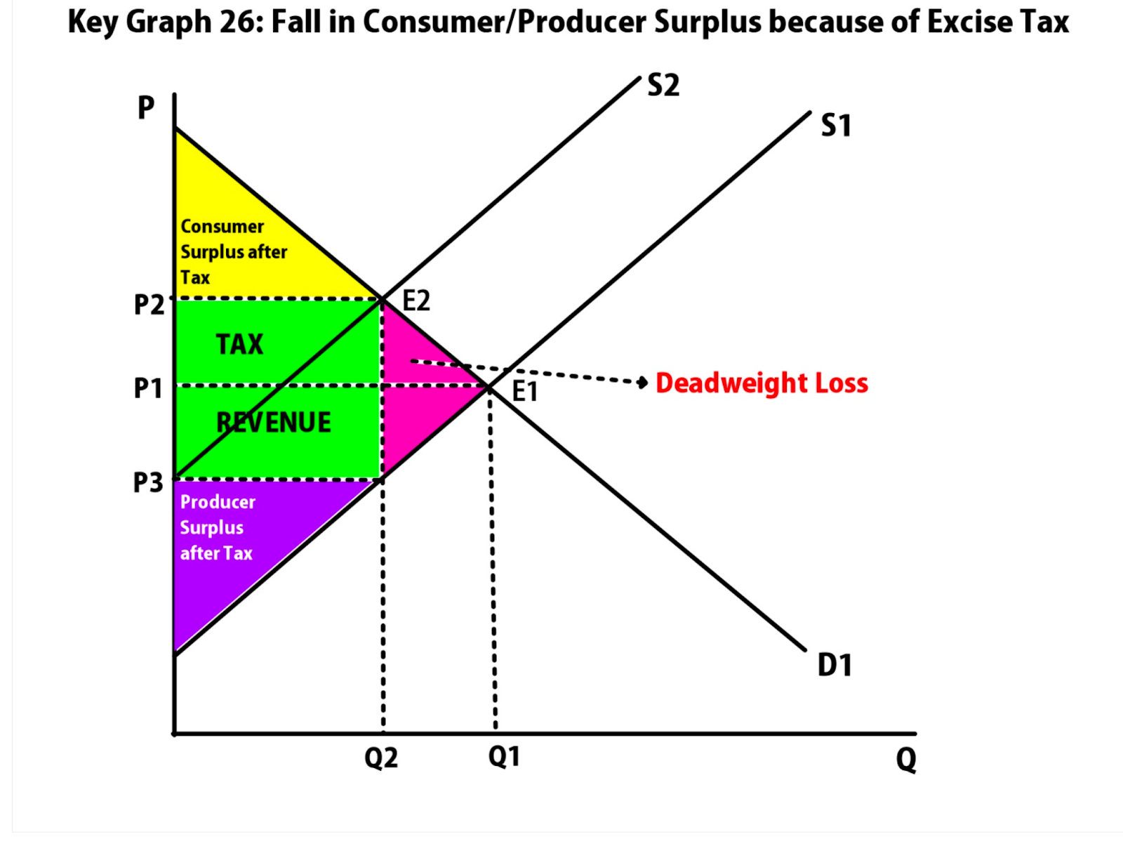
Deadweight loss (DWL) : transactions that should occur, but don’t because of government intervention (calculate the area = triangle formula, ½(base x height)
2.7 - Market Disequilibrium and Changes in Equilibrium
2.8 - Government Intervention in Markets
Market Disequilibrium:
Shortage : Qs < Qd, price is lower than equilibrium
Surplus : Qs > Qd, price is above equilibrium
Price floor : minimum price a supplier can charge, price is set above equilibrium (causes shortage)
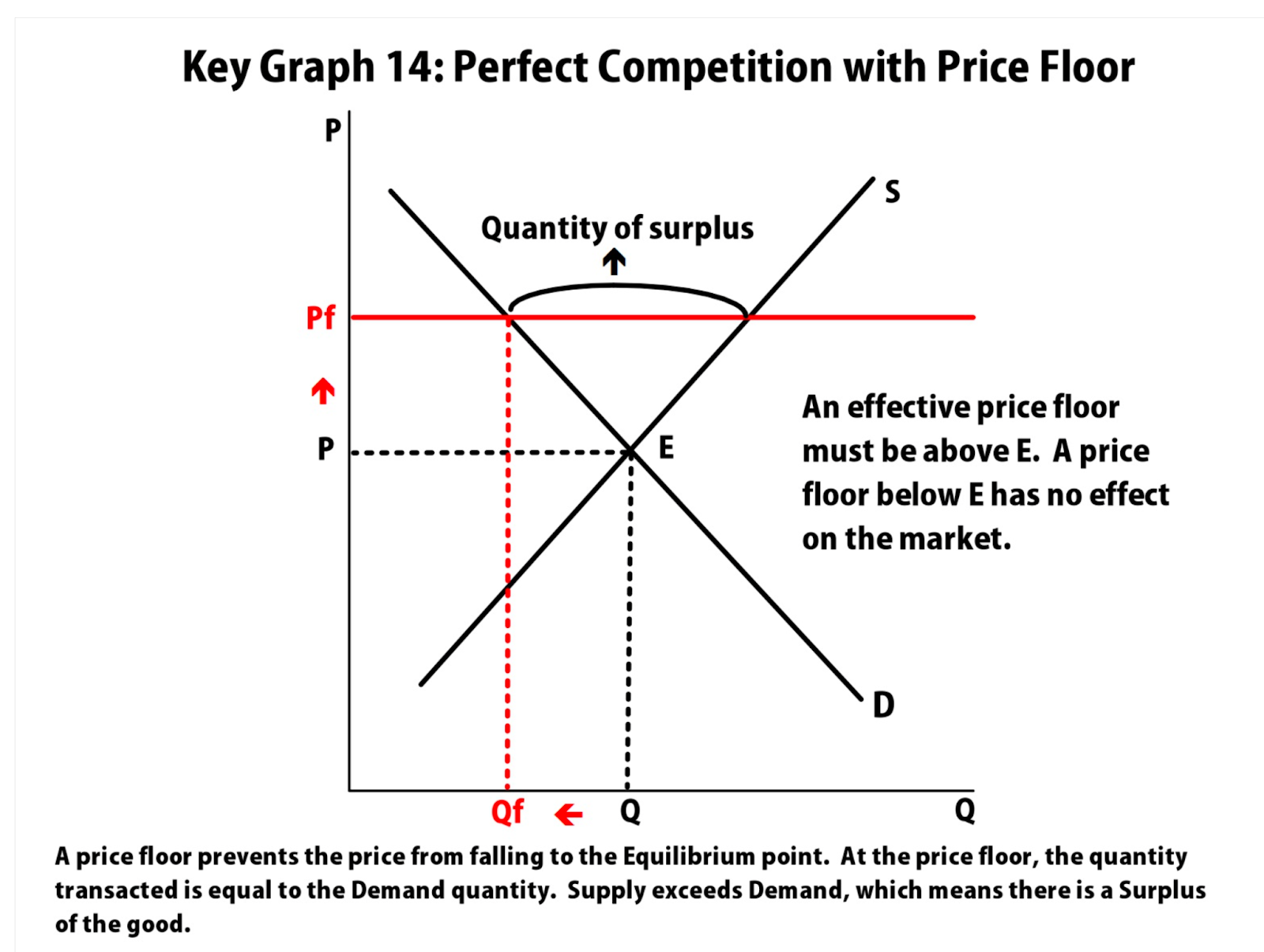
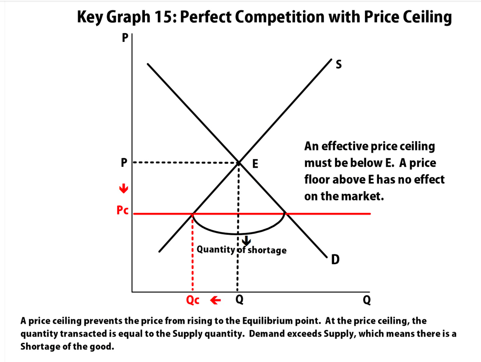
Price ceiling : maximum price a supplier can charge, price is set below equilibrium (causes surplus)
Quota : upper limit of a quantity that can be bought or sold (known as quantity control)
License : gives an owner the right to supply a good/service
Demand price : the price at which consumers will demand that quantity
Supply price : the price at which producers will supply that quantity
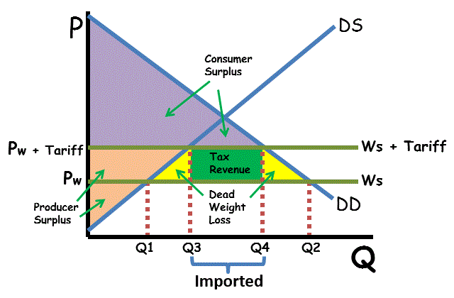
2.9 - International Trade and Public Policy
Quota rent : difference between demand price and supply price
Tariffs : tax placed on a good that is imported or exported
Import quota : restriction on the quantity of a good that can be imported
Unit 3 - Production, Cost, and the Perfect Competition Model
3.1 - The Production Function
Production function : relation between the quantity of inputs a firm uses and the quantity of output it produces.
Also related to how firms produce goods using the factors of production (land, labor, capital, and entrepreneurship)
Some terms you will encounter a lot:
Fixed input : an input whose quantity doesn’t change
Variable input : an input whose quantity can change
Long run : time period in which all inputs can be variable
Short run : time period in which at least 1 input is fixed
Marginal product : change in overall output when input changes
Marginal product of labor (MPL) : ∆Q/∆L
Diminishing marginal returns : as input increases, the output of each input will be less than the previous input
Output : quantity produced
Rental rate : price of capital
Capital : goods that are used to produce goods/services
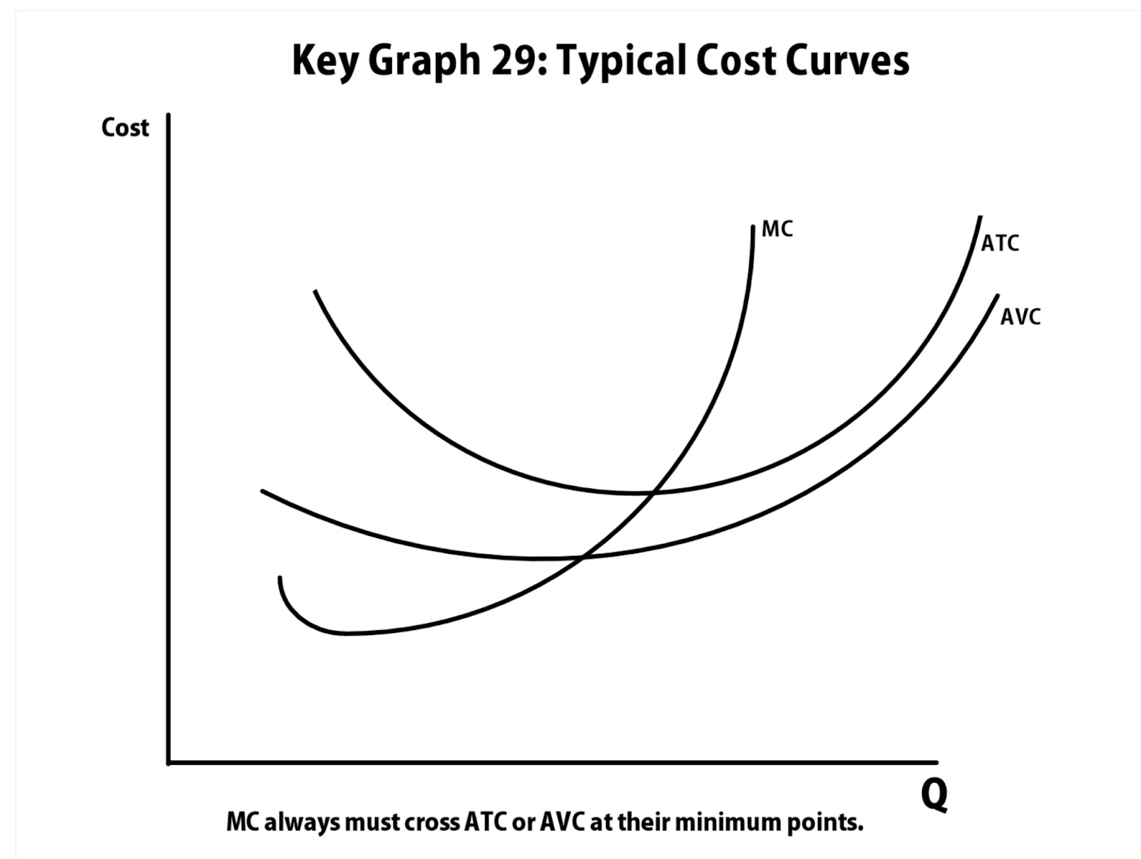
3.2 - Short-Run Production Costs
This portion aims to look into how costs change depending on quantity in the short run. The short run is the period in which at least one of our inputs are fixed. On the other hand, the long run looks into costs which aim to minimise our costs.
This can be measured by understanding the following concepts
Fixed cost : cost that doesn’t change with amount of output produced (ex. oven)
Variable cost : cost that changes with amount of output produced
Total cost : fixed cost + variable cost
Marginal cost : cost difference of one additional unit of output (∆TC/∆Q)
Average fixed cost (AFC) : FC/Q
Average variable cost (AVC) : VC/Q
Average total cost (ATC) : TC/Q
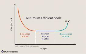
3.3 - Long-Run Production Costs
In the long run, all inputs are variable, which is where the firms aims to adjust to minimise costs regardless of what short run average total cost curve it is on.
Long run average total cost (LRATC) : same as short run ATC, but bigger
Economies of scale : LRATC declines as output increases
Diseconomies of scale : LRATC increaess as output increases
Constant returns to scale : output increase directly in proportion to an increase in all inputs (ex. input doubles, output also doubles)
3.4 - Types of Profit
As we know, there are concepts such as revenue, gains, and costs, which are all different than profit. Profit is the excess revenue that a business gets to keep.
Economic profit : revenue - explicit cost - implicit cost, or accounting profit - implicit cost
Accounting profit : revenue - explicit cost
Implicit cost : not an actual cost, a cost that you could’ve been earning (ex. if you own a restaurant, the implicit cost would be the salary you would have earned as being a chef working in a different restaurant)
Marginal Revenue: additional revenue gained by producing one more unit
3.5 - Profit Maximisation
The profit Maximising point for a firm is where it aims to increase revenue due to costs possibly being high as well.
MR = MC
If you cannot have MR=MC, MR>MC
The firms aim to produce where MR = MC due to the fact that all profits are earned without overshooting and gathering additional costs.
These calculations help a firm understand how much it must produce in order to maximise their profits.
3.6 - Firm’s’ Short-Run Decision to Produce and Long-Run Decisions to Enter or Exit a Market
Firms need to be able to know when to enter the market, as well as when to end production (entry and exit). By understanding profits, we are able to know what a firm does and therefore how many quantities to produce.
Short Run:
Shutdown rule : as long as P > AVC, continue to produce
If AVC > P : shutdown
Firms can make profit or losses
Long Run :
Exit rule : if P < ATC, exit the market
Firms make normal profit ($0), unless monopoly or oligopoly
Shut down rule: a firm should not produce unless it can cover its variable costs. If it is not able to do so, firms are better off producing nothing. However, this only tends to happen in perfect competition)
Perfect competition occurs when P<AVC at MR = MC)
As a result, this leads to long term adjustments in the long run where equalities in the market make a normal profit
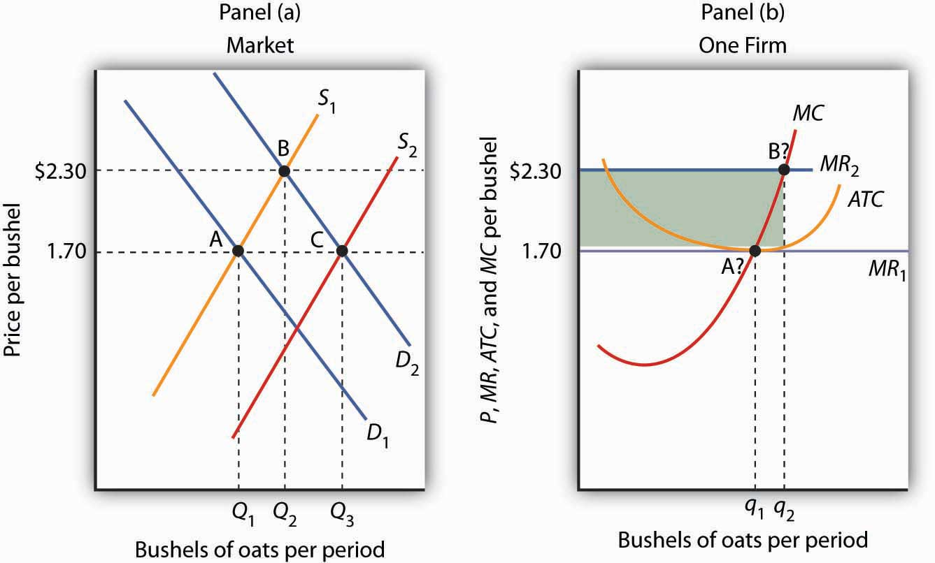
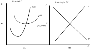
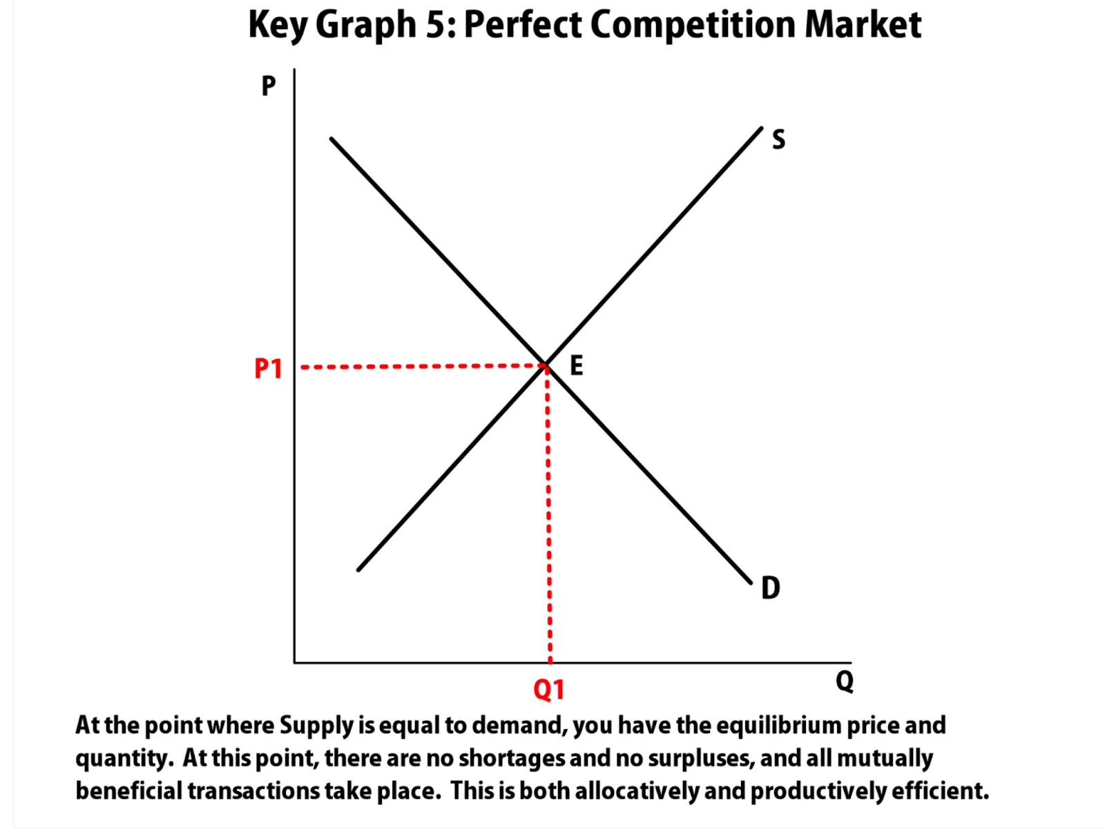
3.7 Perfect Competition
In perfect competition, many identical firms are competing at a constant market price. This market has low barriers, meaning any firm is able to enter and exit the market in the long run.
Firms in this market are price takers, who are firms which cannot charge a higher price than the equilibrium price. This means that they have no market power.
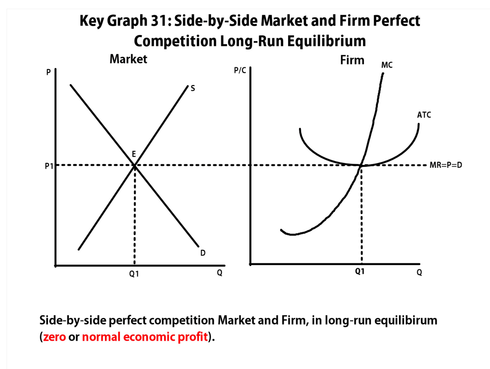
Long run will have normal profit
Short run can have either profit or loss
Unit 4 - Imperfect Competition
4.1 - Introduction to Imperfectly Competitive Markets
Firms are able to make an increased profit in the long run if there is less competition since firms are considered to be price makers. There are stricter barriers to entry in imperfect competition (Governmental, economies of scale, geography, and so on)
Common barriers to entry: control of scarce resources, legal barriers, high startup costs
Perfect Competition | Monopolistic Competition | Monopoly | Oligopoly | |
|---|---|---|---|---|
# of firms | Many | Many | 1 | Few |
Type of product | Standard | Differentiated | Unique | Standard or different |
Price control | None | Little | Yes | Some |
Barriers to entry | None | None (few) | High | High |
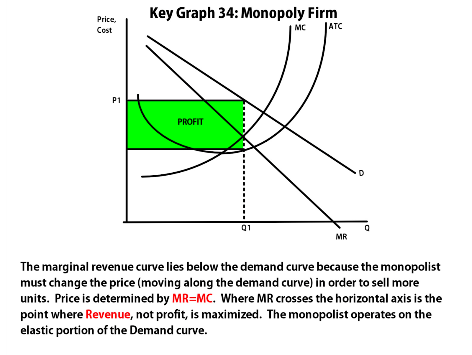
4.2 - Monopolies
Monopoly: market structure where there is only one firm producing a product
Only producer of a good, has no close substitutes
On the graph, there is a downward sloping demand curve
Quantity is produced : at MR = MC
Price is : MR=MC, up to demand
Supply curve : where MC > AVC
Allocatively efficient due to them producing at MR=MC
Productively inefficient because they don’t produce at the minimum of the ATC
Natural monopoly: has large fixed costs, and long economies of scale, has downward sloping ATC curve
Natural monopoly production point : MR=MC
Government will correct by forcing them to set price : at ATC=D
4.3 - Price Discrimination
Price discrimination occurs in specific industries as consumers pay a different price for the same good.
To be able to price discriminate, you need market power
Imperfect price discrimination : charging consumers different prices based on the buyer’s willingness to pay
Perfect price discrimination : charges all consumers the maximum they are willing to pay, no deadweight loss, produce at P=MC
Example : resellers, coupons, bulk buying (costco), etc.
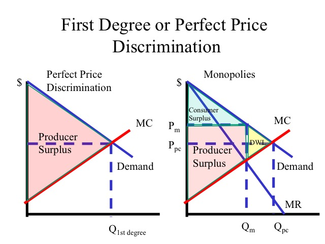
In price discrimination, there is no deadweight loss and no consumer surplus as well, only producer surplus.
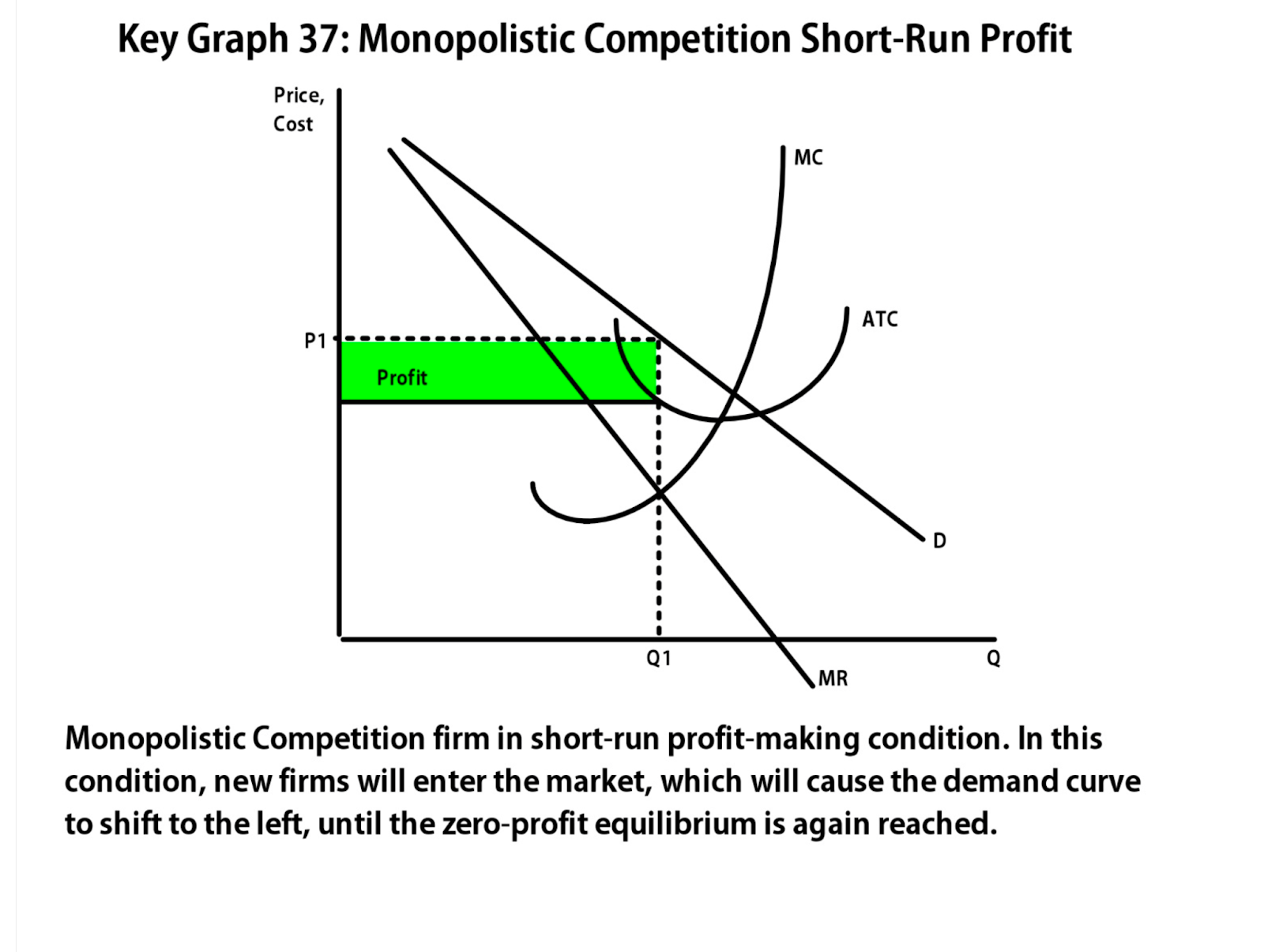
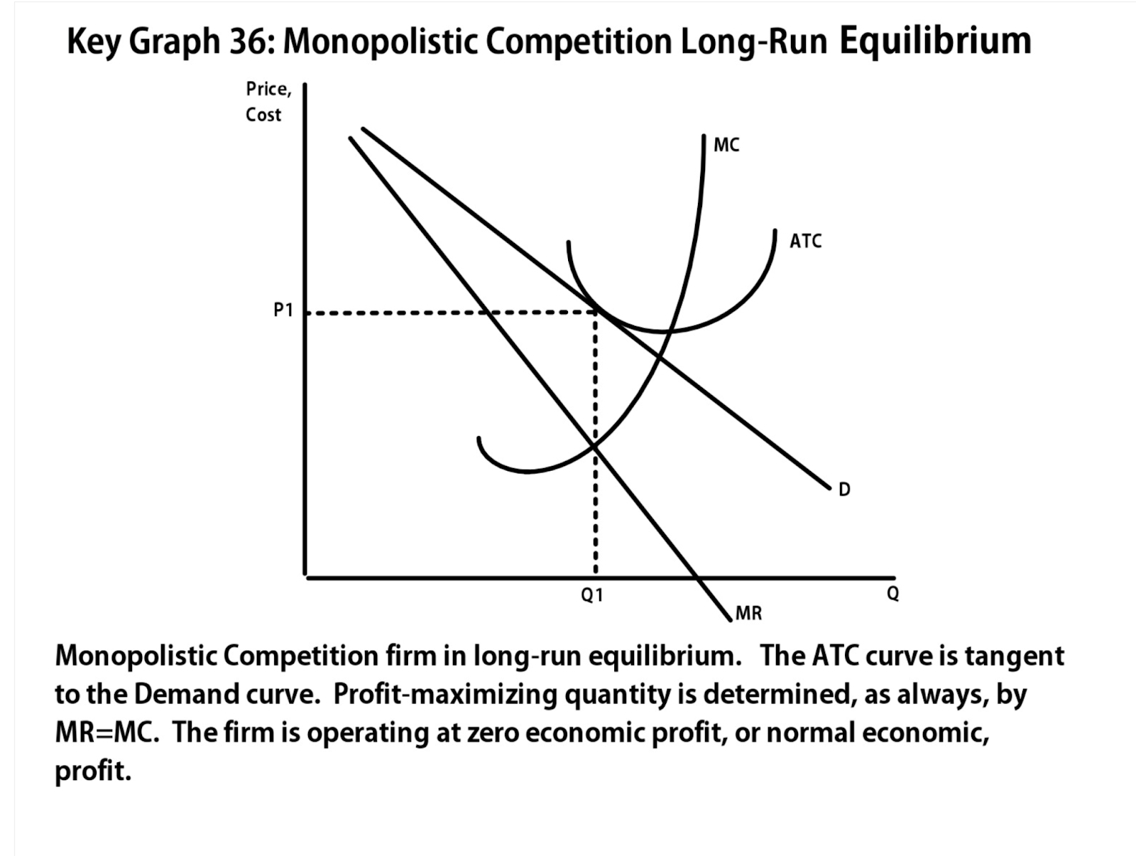
4.4 - Monopolistic Competition
Monopolistic competition: is another term for imperfect competition, and occurs when many companies offer competing products which are similar but not perfect substitutes.
Characteristics:
Combines features of both a monopoly and perfect competition
Many sellers and differentiated products
Will use advertising to make demand more inelastic + differentiate product
Makes profit in short run, normal profit in long run
Allocatively inefficient (P does not equal MC)
Productively inefficient (does not produce @ minimum of ATC, until long run)
Downwards sloping demand curve
Produce at MR = MC, price is MR = MC up to demand
Long Run
Normal profit in long run
Short run profits will attract new firms to join, which decreases the demand until the demand Curve is tangent to ATC, causing normal profits in long run
In long run, they produce in region where economies of scales exist, because they produce in declining portion of ATC
4.5 - Oligopoly and Game theory
Oligopoly Characteristics
Small number of firms, standard or differentiated product
Interdependent : all the actions that a firm takes will affect the other firms in the oligopoly (if They ask why the market is an oligopoly, say it’s because they’re interdependent)
Cartels : a group that agrees to control the price and output of a product (often form in oligopoly)
Collusion : working together to maximize profit
Graph is almost identical to monopoly (you will never be asked to draw them)
Also produce same quantity and price of monopoly
Game Theory
Payoff matrix : represents the payoff to each player to show combinations of given strategies
Dominant strategy : the strategy that has a better payoff regardless of what strategy the opponent chooses
Nash equilibrium : point where both players can do no better than the other given the choice of their opponent
Unit 5 - Factor Markets
5.1 - Introduction to Factor Markets
Factor markets: is a resource for companies to buy what the need to produce their goods and services
Derived demand : the demand from a resource is derived by product demand
Marginal revenue product (MRP) : the additional revenue that is generated by an additional resource/worker
Marginal factor cost (MFC) : the additional cost of an additional resource/worker
Least cost rule : marginal product of labor/price of labor = marginal product of capital/price of capital (MPL/PL=MPK/PK)
Buy more of the one with a higher sum, and less of the one with a smaller sum (to explain, as you increase, diminishing marginal returns kicks in)
5.2 - Changes in Factor Demand and Factor Supply
Determinants of Labor Demands (DL) | Determinants of Labor Supply (SL) |
|---|---|
R.O.D | P.I.N |
1. Productivity of the Resource | 1. Personal values |
2. Price of Other resources | 2. Intervention by Government |
3. Product demand | 3. Number of Qualified workers |
These factors determine the supply and demand of these quantities
5.3 - Profit-Maximising Behaviour in Perfectly Competitive Factor Markets
Market curve : standard supply and demand curve
Equilibrium wage in the market : establishes the wage that firms will pay workers
MRP=MRC!!!!
Firms will not hire if MRC>MRP, as they will be at a loss
5.3 - Monopsonistic Markets
Many sellers, one buyer
Monopsonies pay a lower wage and hire less than perfect competition
This market is an example of Imperfect competition
MRP=MFC
MFC > supply
Unit 6 - Market Failure and the Role of Government
6.1 Socially Efficient and Inefficient Market Outcomes
Socially efficiency is when resources are allocated effectively
MSB=MSC !!
Allocatively Efficient Points
Perfectly competitive market : S=D, MB=MC
Perfectly competitive firm : P=MC
Perfectly competitive labor market : W=MRP (total economic surplus : MSC=MSB)
Causes of Market Failure
Market power (imperfectly competitive markets)
Asymmetric information (lack of info provided by buyers and sellers)
Positive and negative externalities
Insufficient production of public goods
Government policies used to get rid of DWL
Taxes
Subsidies
Reguations
Public prodivions
Market failure : exists when firms produce @ MPC=MPC, S=D
The government tries to get them to produce @ MSC =MSB
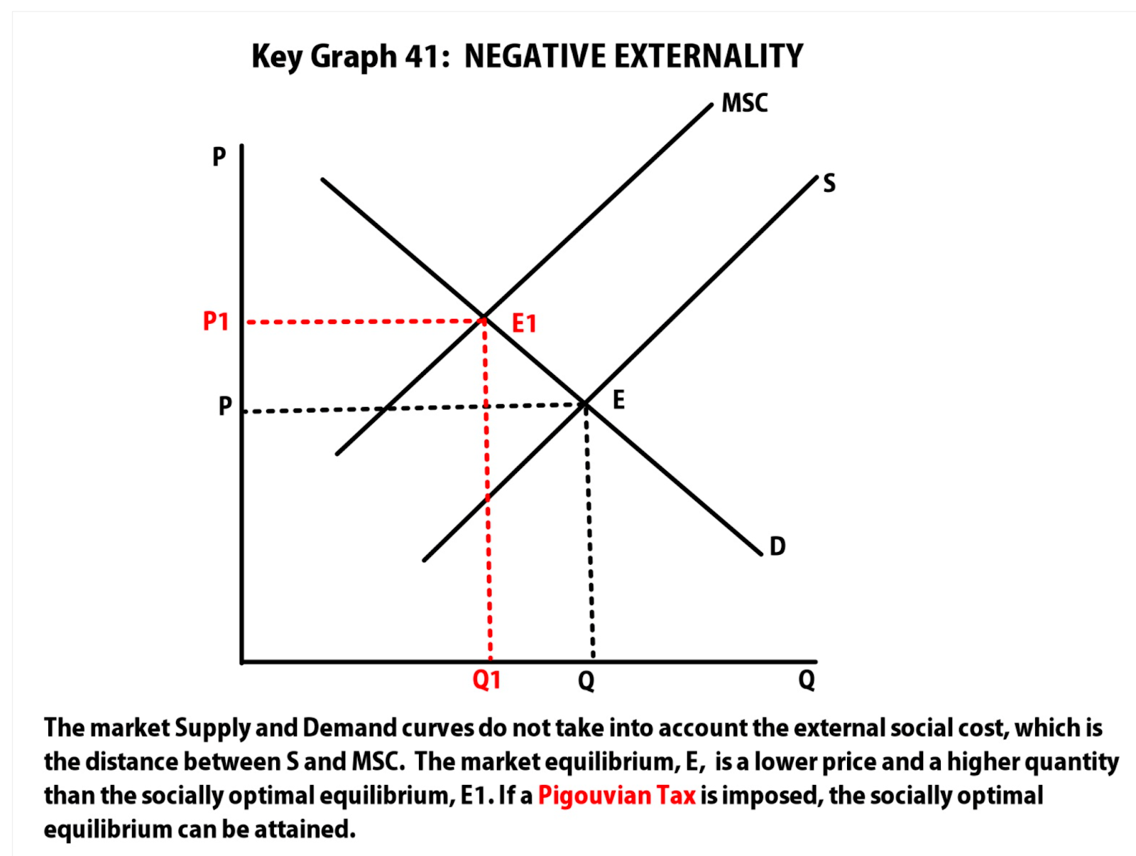
6.2: Externalities
Externality : when external cost/benefit is placed on members of society who did not pay for them
MSB does not equal MSC
Negative externality : when someone uses a product, it decreases the benefit of others (ex. smoking), MSC > MPC (correct with per unit tax)
Positive externality : when one uses a product, others benefit (ex. education) MSC < MPC (correct with subsidy)
6.3: Public and Private Goods
Rivalrous good : if someone consumers a product, others cannot
Rivalrous : food, shoes, etc
Nonrivalrous : national defense, fireworks, etc
Somewhere in middle : schools, roads, etc
Excludable good : non payers can be prevented from enjoying the benefits
Excludable : food, school, etc
Nonexcludable : national defense, air, etc
Public goods : underproduced due to freeloader problem
Examples : national defense, law enforcement, etc
Freeloader problem : people can enjoy the benefit of a good/service without paying
Government will provide subsidies to producers
Private goods : goods produced by private markets, can be excludable
6.4: The Effects of Government Intervention in Different Market Structures
Causes of inefficient markets
Market power
Externalities
Nonrival and nonexcludable goods (public goods)
Forms of government intervention
Taxes
Subsidies
Price floors/ceilings
Regulation
Per unit subsidy : gives benefits per unit
Perfect competition : MC, ATC, AVC decreases, price doesn’t change (price taker)
Monopolistic competition : MC, ATC, price decreases (price maker @ MR=MC)
Lump sum subsidy : gives benefit no matter how many units
Taxes will always shift supply curve to the left in long run, profits decrease
Per unit tax : increase MC, ATC, and AVC
Perfect competition : MC, ATC, AVC increases, price doesn’t change (price taker)
Monopolistic competition : MC, ATC, price increases (price maker @ MR=MC)
Lump sum tax : only increase ATC
won’t change output level
Non price regulation : works like taxes, they ensure competition/environmental protection/health and safety
Antitrust policy : promote competition and prevents monopolies
Antitrust laws
Lawsuits
Price controls
Subsidies
Price ceiling : sets minimum price
Perfect competition : causes shortage
Monopolistic competition : becomes MR curve, price and output decreases
Price floor : sets maximum price
Perfect competition : leads to surplus
Monopsony : wages go up and workers go up
6.5: Inequality
Income distribution : measures % of income that goes to individuals in different percentiles/brackets
In a system with perfectly equality : everyone would receive equal shares of income
Income : wages, rent, interest, profit
Lorenz curve : measures the distribution of income equality (you want to be as close of possible to the perfect equality line as possible)
Gini coefficient : A/(A+B)
Closer to 0, more equality
Closer to 1, the more inequality
Causes of income inequality
Supply + demand in labor market
Human capital
Discrimination
Inheritance
Bargaining power
Etc
Policies to address inequality
Taxes + transfers
Minimum wage laws
Anti-poverty program
Income protection program
Scholarships
Taxes :
Proportional : everyone pays the same percentage of their income (no impact on income distribution)
Progressive : taxes are higher % on people earning a higher income (reduces income inequality)
Regressive : taxes are lower % on people earning a higher income (increases income inequality)