


Chapter 4: Applications of Differential Calculus
A. Slope; Critical Points
If the derivative of y = f (x) exists at P(x1, y1), then the slope of the curve at P (which is defined to be the slope of the tangent to the curve at P) is f′(x1), the derivative of f(x) at x = x1.
Any c in the domain of f such that either f′(c) = 0 or f′(c) is undefined is called a critical point or critical value of f. If f has a derivative everywhere, we find the critical points by solving the equation f′(x) = 0.
Example:
Solution:
Average and Instantaneous Rates of Change
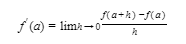
If as x varies from a to a + h, the function f varies from f(a) to f(a + h), then we know that the difference quotient

is the average rate of change of f over the interval from a to a + h.
The average velocity of a moving object over some time interval is the change in distance divided by the change in time.
The average rate of growth of a colony of fruit flies over some interval of time is the change in size of the colony divided by the time elapsed.
The average rate of change in the profit of a company on some gadget with respect to production is the change in profit divided by the change in the number of gadgets produced.
The (instantaneous) rate of change of f at a, or the derivative of f at a, is the limit of the average rate of change as h → 0:
On the graph of y = f(x), the rate at which the y-coordinate changes with respect to the x-coordinate is f′(x), the slope of the curve.
The rate at which s(t), the distance traveled by a particle in t seconds, changes with respect to time is s′(t), the velocity of the particle.
The rate at which a manufacturer’s profit P(x) changes relative to the production level x is P′(x).
Example:
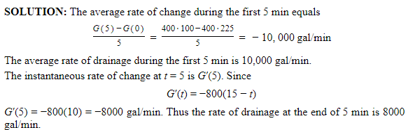
Let G = 400(15 − t)² be the number of gallons of water in a cistern t minutes after an outlet pipe is opened. Find the average rate of drainage during the first 5 minutes and the rate at which the water is running out at the end of 5 minutes.
Solution:
B. Tangents to a Curve
An equation of the tangent to the curve y = f(x) at point P(x1, y1) is
y − y1 = f′(x1)(x − x1)
If the tangent to a curve is horizontal at a point, then the derivative at the point is 0.
If the tangent is vertical at a point, then the derivative does not exist at the point.
Example:
Find an equation of the tangent to the curve of f(x) = x³ − 3x² at the point (1,−2).
SOLUTION:
Since f′(x) = 3x² − 6x and f′(1) = −3, an equation of the tangent is
y + 2 = −3(x − 1) or y + 3x = 1
C. Increasing and Decreasing Functions
Functions with Continuous Derivatives
A function y = f(x) is said to be increasing/decreasing on an interval if for all a and b in the interval such that a<b, f(b)≥f(a) / f(b)≤f(a). To find intervals over which f(x) increasing/decreasing, that is, over which the curve rises/falls, analyze the signs of the derivative to determine where f′(x)≥0/f′(x)≤0.
Example:
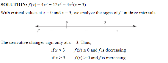
For what values of x is f(x) = x⁴ − 4x³ increasing and for what values is it decreasing?
Solution:
Functions with Discontinuous Derivatives
Here we proceed as in Case I, but also consider intervals bounded by any points of discontinuity of f or f′
Example:
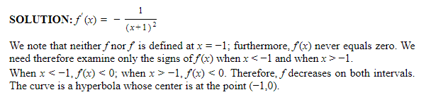
For what values of x is f(x)=1 / x+1 increasing and for what values is it decreasing?
Solution:
D. Maximum, Minimum, Concavity, and Inflection Points: Definition
The curve of y = f(x) has a local (or relative) maximum/minimum at a point where x = c if
f(c)⩾f(x) / f(c)⩽f(x)for all x in the immediate neighborhood of c.
If a curve has a local maximum/minimum at x = c, then the curve changes from rising/falling to falling/rising as x increases through c.
If a function is differentiable on the closed interval [a,b] and has a local maximum or minimum at x = c (a < c < b), then f′(c) = 0. The converse of this statement is not true.
If f(c) is either a local maximum or a local minimum, then f(c) is called a local extreme value or local extremum. (The plural of extremum is extrema.)
The global or absolute maximum/minimumof a function on [a,b] occurs at x = c if f(c)⩾f(x) / f(c)⩽f(x) for all x on [a,b].
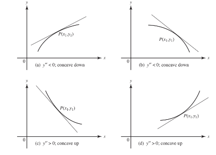
A curve is said to be concave upward/downward on an interval (a,b) if the curve lies above/below the tangent lines at each point in the interval (a,b). If y″>0 y″<0 at every point in an interval (a,b), the curve is concave up/down.
E. Maximum, Minimum, Concavity, Inflection Points: Curve Sketching
Functions that are everywhere differentiable
The following procedure is suggested to determine any maximum, minimum, or inflection point of a curve and to sketch the curve:
Find y′ and y″.
Find all critical points of y, that is, all x for which y′ = 0. At each of these x’s the tangent to the curve is horizontal.
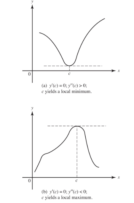
Let c be a number for which y′ is 0; investigate the sign of y″ at c. If y″(c) > 0, then c yields a local minimum; if y″(c) < 0, then c yields a local maximum. This procedure is known as the Second Derivative Test (for extrema). If y″(c) = 0, the Second Derivative Test fails and we must use the test in step (4), which follows.
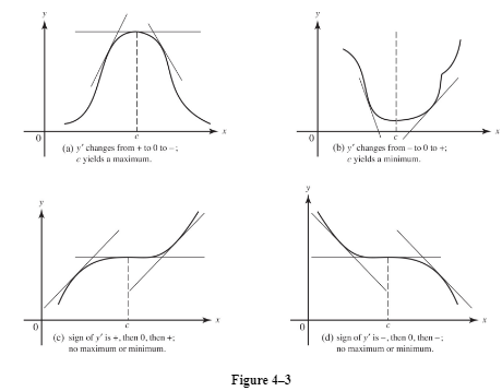
If y′(c) = 0 and y″(c) = 0, investigate the signs of y′ as x increases through c. If y′(x) > 0 for x’s (just) less than c but y′(x) < 0 for x’s (just) greater than c, then the situation is that indicated in (a) of Figure 4–3, where the tangent lines have been sketched as x increases through c; here c yields a local maximum. If the situation is reversed and the sign of y′ changes from − to + as x increases through c, then c yields a local minimum. In Figure 4–3, (b) shows this case. The schematic sign pattern of y′, + 0 − or − 0 +, describes each situation completely. If y′ does not change sign as x increases through c, then c yields neither a local maximum nor a local minimum. Two examples of this appear in (c) and (d) of Figure 4–3.
Find all x’s for which y″ = 0; these are x-values of possible points of inflection. If c is such an x and the sign of y″ changes (from + to − or from − to +) as x increases through c, then c is the x-coordinate of a point of inflection. If the signs do not change, then c does not yield a point of inflection.
The crucial points found as indicated in (1) through (5) above should be plotted along with the intercepts. Care should be exercised to ensure that the tangent to the curve is horizontal whenever dydx=0 and that the curve has the proper concavity.
Example:
Sketch the graph of f(x) = x⁴ − 4x³.
SOLUTION:
f′(x) = 4x³ − 12x² and f″(x) = 12x² − 24x.
f′(x) = 4x²(x − 3), which is zero when x = 0 or x = 3.
Since f″(x) = 12x(x − 2) and f″(3) > 0 with f′(3) = 0, the point (3,−27) is a local minimum. Since f″(0) = 0, the Second Derivative Test fails to tell us whether x = 0 yields a local maximum or a local minimum.
Since f′(x) does not change sign as x increases through 0, the point (0,0) yields neither a local maximum nor a local minimum.
f″(x) = 0 when x is 0 or 2; f 0 changes signs as x increases through 0 (+ to −), and also as x increases through 2 (− to +). Thus both (0,0) and (2,−16) are inflection points of the curve.

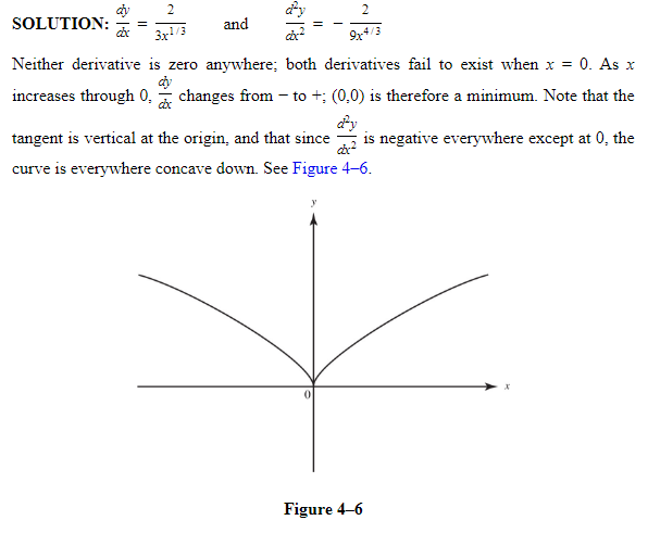
Functions Whose Derivatives May Not Exist Everywhere
If there are values of x for which a first or second derivative does not exist, we consider those values separately, recalling that a local maximum or minimum point is one of transition between intervals of rise and fall and that an inflection point is one of transition between intervals of upward and downward concavity.
Example:
Solution:
F. Global Maximum or Minimum
Differentiable Functions
If a function f is differentiable on a closed interval a ⩽ x ⩽ b, then f is also continuous on the closed interval [a,b] and we know from the Extreme Value Theorem that f attains both a (global) maximum and a (global) minimum on [a,b].
To find these, we solve the equation f′(x) = 0 for critical points on the interval [a,b], then evaluate f at each of those and also at x = a and x = b.
The largest value of f obtained is the global max, and the smallest the global min.
This procedure is called the Closed Interval Test**, or the** Candidates Test.
Example :
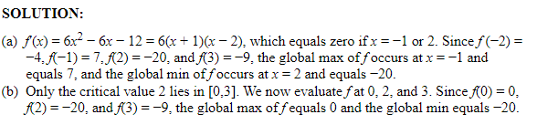
Find the global max and global min of f on (a) −2 ⩽ x ⩽ 3, and (b) 0 ⩽ x ⩽ 3, if f(x) = 2x³ − 3x² − 12x.
SOLUTION:
Functions that are not everywhere Differentiable
We proceed as for Case I but now evaluate f also at each point in a given interval for which f is defined but for which f′ does not exist.
Example:
The absolute-value function f(x) = |x| is defined for all real x, but f′(x) does not exist at x = 0. Since f′(x) = −1 if x < 0, but f′(x) = 1 if x > 0, we see that f has a global min at x = 0.
G. Further Aids in Sketching
It is often very helpful to investigate one or more of the following before sketching the graph of a function or of an equation:
Intercepts. Set x = 0 and y = 0 to find any y- and x-intercepts, respectively.
Symmetry. Let the point (x,y) satisfy an equation. Then its graph is symmetric about
the x-axis if (x,−y) also satisfies the equation
the y-axis if (−x,y) also satisfies the equation
the origin if (−x,−y) also satisfies the equation
Asymptotes. The line y = b is a horizontal asymptote of the graph of a function f if either limx→∞f(x)=b or limx→∞f(x)=b. If f(x)=P(x)Q(x), inspect the degrees of P(x) and Q(x), then use the Rational Function Theorem. The line x = c is a vertical asymptote of the rational function P(x)Q(x) if Q(c) = 0 but P(c) ≠ 0.
Points of discontinuity. Identify points not in the domain of a function, particularly where the denominator equals zero.
Example :
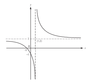
Sketch the graph of y=2x+1x−1.
SOLUTION:
If x = 0, then y = −1. Also, y = 0 when the numerator equals zero, which is when x=−1/2. A check shows that the graph does not possess any of the symmetries described previously. Since y → 2 as x → ±∞, y = 2 is a horizontal asymptote; also, x = 1 is a vertical asymptote. The function is defined for all reals except x = 1; the latter is the only point of discontinuity.
We find derivatives:
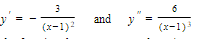
From y′ we see that the function decreases everywhere (except at x = 1), and from y″ that the curve is concave down if x < 1, up if x > 1.
H. Optimization: Problems involving Maxima and Minima
The techniques described above can be applied to problems in which a function is to be maximized (or minimized).
Often it helps to draw a figure.
If y, the quantity to be maximized (or minimized), can be expressed explicitly in terms of x, then the procedure outlined above can be used.
If the domain of y is restricted to some closed interval, one should always check the endpoints of this interval so as not to overlook possible extrema.
Often, implicit differentiation, sometimes of two or more equations, is indicated.
Example:
The region in the first quadrant bounded by the curves of y2 = x and y = x is rotated about the y-axis to form a solid. Find the area of the largest cross section of this solid that is perpendicular to the y-axis.
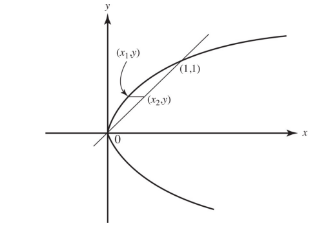
Solution:
I. Relating a Functions and its Derivatives Graphically
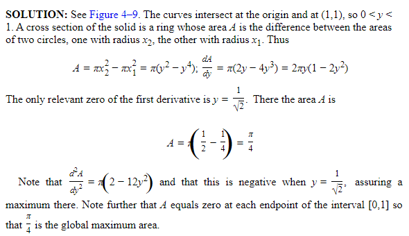
The following table shows the characteristics of a function f and their implications for f’s derivatives.
These are crucial in obtaining one graph from another. The table can be used reading from left to right or from right to left.
Note that the slope at x = c of any graph of a function is equal to the ordinate at c of the derivative of the function.
If f′(c) does not exist, check the signs of f′ as x increases through c: plus-to-minus yields a local maximum; minus-to-plus yields a local minimum; no sign change means no maximum or minimum, but check the possibility of a point of inflection.
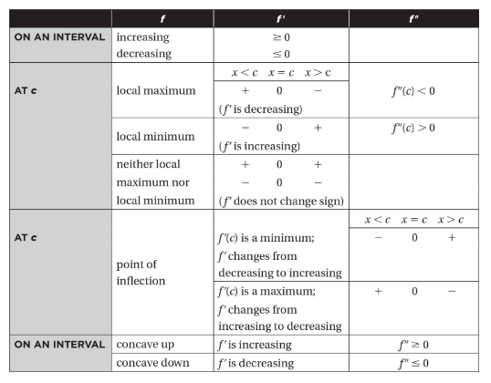
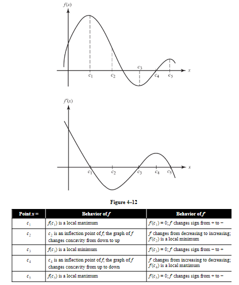
Example:
Given the graph of f(x) shown in Figure 4-12 sketch f′(x).
J. Motion along a Line
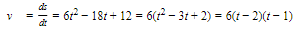
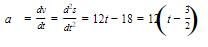
If a particle moves along a line according to the law s = f(t), where s represents the position of the particle P on the line at time t, then the velocity v of P at time t is given by ds/dt and its acceleration a by dv/dt or by d2s/dt2.
The speed of the particle is |v|, the magnitude of v.
If the line of motion is directed positively to the right, then the motion of the particle P is subject to the following: At any instant,
if v > 0, then P is moving to the right (its position s is increasing); if v < 0, then P is moving to the left (its position s is decreasing)
if a > 0, then v is increasing; if a < 0, then v is decreasing
if a and v are both positive or both negative, then (1) and (2) imply that the speed of P is increasing or that P is accelerating; if a and v have opposite signs, then the speed of P is decreasing or P is decelerating
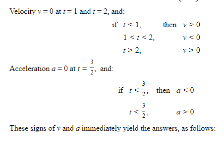
if s is a continuous function of t, then P reverses direction whenever v is zero and a is different from zero; note that zero velocity does not necessarily imply a reversal in direction
Example :
A particle moves along a horizontal line such that its position s = 2t3 − 9t2 + 12t − 4, for t ≧ 0.
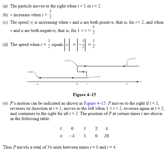
Find all t for which the particle is moving to the right.
Find all t for which the velocity is increasing.
Find all t for which the speed of the particle is increasing.
Find the speed when t=32.
Find the total distance traveled between t = 0 and t = 4.
Solution:
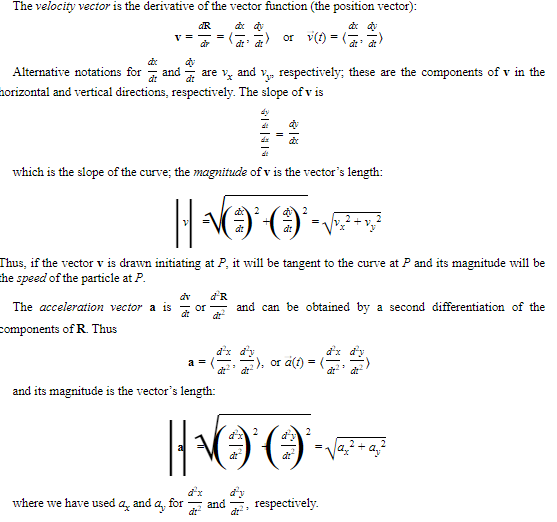
K. Motion along a Curve: Velocity and Acceleration Vectors
If a point P moves along a curve defined parametrically by P(t) = (x(t), y(t)), where t represents time, then the vector from the origin to P is called the position vector, with x as its horizontal component and y as its vertical component.
The set of position vectors for all values of t in the domain common to x(t) and y(t) is called the vector function.
A vector may be symbolized either by a boldface letter (R) or an italic letter with an arrow written over it (→R) The position vector, then, may be written as →R(t)=〈x,y〉 or as R = 〈x,y〉.
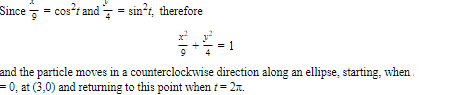
Example :
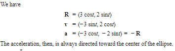
A particle moves according to the equations x = 3 cos t, y = 2 sin t.
Find a single equation in x and y for the path of the particle and sketch the curve.
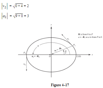
Find the velocity and acceleration vectors at any time t, and show that a = −R at all times.
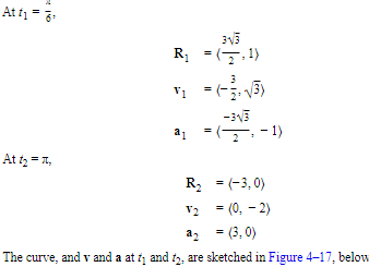
Find R, v, and a when (1) t1=π6, (2) t2 = π, and draw them on the sketch.
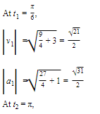
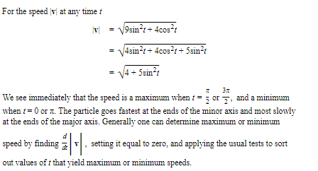
Find the speed of the particle and the magnitude of its acceleration at each instant in 3.
When is the speed a maximum? When is the speed a minimum?
SOLUTIONS:
L. Tangent-Line Approximation
If f′(a) exists, then the local linear approximation of f(x) at a is
f(a) + f′(a)(x − a)
Since the equation of the tangent line to y = f(x) at x = a is
y − f(a) = f′(a)(x − a)
we see that the y value on the tangent line is an approximation for the actual or true value of f. Local linear approximation is therefore also called tangent-line approximation. For values of x close to a, we have
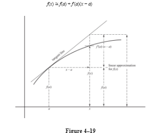
where f(a) + f′(a)(x − a) is the linear or tangent-line approximation for f(x), and f′(a)(x − a) is the approximate change in f as we move along the curve from a to x.
In general, the closer x is to a, the better the approximation is to f(x).
Example:
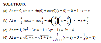
Find tangent-line approximations for each of the following functions at the values indicated:
sin x at a = 0
cosx at a=π2
2x3 − 3x at a = 1
√1+x at a=8
SOLUTIONS:
M. Related Rates
If several variables that are functions of time t are related by an equation, we can obtain a relation involving their (time) rates of change by differentiating with respect to t.
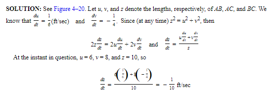
Example:
If several variables that are functions of time t are related by an equation, we can obtain a relation involving their (time) rates of change by differentiating with respect to t.
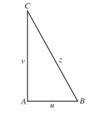
SOLUTION:
N. Slope of a Polar Curve
We know that, if a smooth curve is given by the parametric equations
x = f(t)andy = g(t)
then
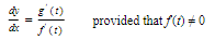
To find the slope of a polar curve r = f(θ), we must first express the curve in parametric form. Since
x = r cos θandy = r sin θ
therefore,
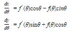
x = f(θ) cos θandy = f(θ) sin θ
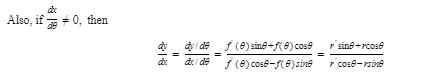
If f(θ) is differentiable, so are x and y; then
Example:
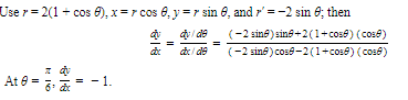
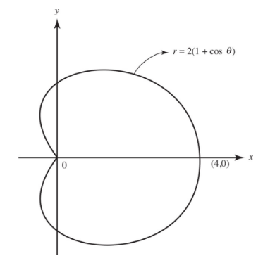
Find the slope of the cardioid r = 2(1 + cos θ) at θ=π/6.
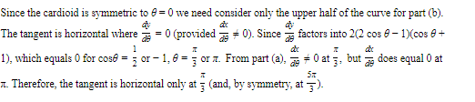
Where is the tangent to the curve horizontal?
Solution: