


Chapter 7: Elasticity, Microeconomics Policy, and Consumer Theory
Elasticity of demand (ED)
It’s a measure of the responsiveness of consumers to change in price
If a firm increases price of their product, would consumers still buy it?
If a demand for a product is inelastic, change in price wouldn’t impact the consumers much e.g. cancer medicines
If the demand for a product is elastic, change in price would impact the quantity purchased of that product
The following is the formula to calculate the ED
%change in Qd / %change in Price
Economists ignore the negative value of PED
The greater the value, the more sensitive consumers are to a change in the price of good X
The answer that is received falls under the following ranges, each with their own interpretation
Type of Elasticity | Elasticity value |
|---|---|
Perfectly inelastic | 0 |
Relatively Inelastic | <1 |
Unit elastic | 1 |
Relatively elastic | >1 |
Perfectly elastic | Infinity |
Example
Suppose the price of designer blue jeans increases from $100 to $120 and the quantity demanded decreases from 10 to 9
First, calculate the percentage change for both price and quantity demanded: ($120 – $100)/$100 = 0.2= 20% increase in price
(9 – 10)/10 = –0.1 = 10% decrease in the quantity demanded.
Ed = (–10%)/(20%) = 0.5
The price elasticity is relatively inelastic
Elasticity on the demand curve
The midpoint formula
(Change in Qd/Change in Price) x (Average price/ Average quantity)
Example
Initial price of a hypothetical product is $16, and 20 units are demanded
The price rises to $20, quantity demanded falls to 10 units.
The average price between these two points is $18, and the average quantity is 15 units
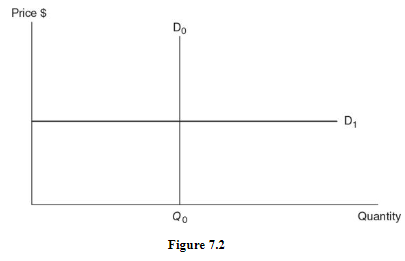
Special cases
The following is a perfectly inelastic demand curve (D0)
No substitutes
Vertical demand curve tells us that no matter what percentage increase, or decrease, in price, the quantity demanded remains the same
Ed = 0
The following is a perfectly elastic demand curve (D1)
Many substitutes
Horizontal demand curve tells us that even the smallest percentage change in price causes an infinite change in the quantity demanded
Ed = infinite
Note: As a demand curve becomes more vertical, the price elasticity falls and consumers become more price inelastic
Determinants of elasticity
Number of Good Substitutes
Proportion of Income
Time
Total revenue test to determine elasticity
Total revenue is price x quantity
The answer falls under the following categories, each with its own interpretation
Type of Elasticity | Relationship between Price and total revenue (TR) |
|---|---|
Relatively elastic | inverse relation |
Relatively inelastic | direct relation |
Unit elastic | TR doesn’t change when P changes |
If price increases but total revenue decreases, the demand for the product is relatively elastic
If price increases and total revenue also increases, the demand for the product is relatively inelastic
If price changes but total revenue stays same, the demand for the product is unit elastic
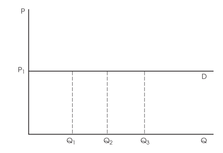
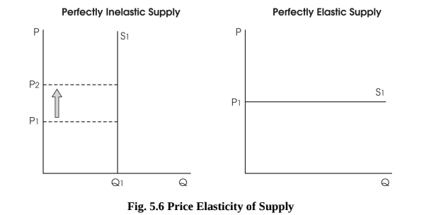
Perfect elasticity
If the demand is perfectly elastic, the price elasticity is infinity
Any price above P1 and the demand falls to zero
Any price that’s exactly P1, the demand could keep increasing (buyers would buy as much quantity as possible)
Any price below P1 and the quantity demanded becomes infinite
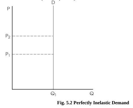
Perfect inelasticity
If the demand is perfectly inelastic, the price elasticity of demand is zero
As the price keeps on changing, the quantity demanded stays same
A good example of this would be life-saving drugs
Prices could increase by a big margin but quantity demanded wouldn’t change still
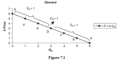
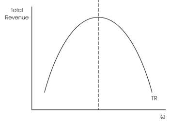
Elasticity along a linear demand curve
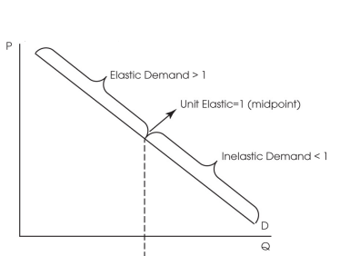
The demand curve is elastic towards the top, unit elastic at the midpoint and inelastic towards the bottom
As the prices decrease in the elastic range, the total revenue eventually increases
As the prices decrease in the inelastic range, the total revenue actually decreases
Monopolies (a type of market structure) prefer producing in the elastic range because that’s also where the revenue is maximized
Income Elasticity of demand
This measure how the demand for a product changes with respect to change in their income
% change in quantity demanded/ %change in consumers income
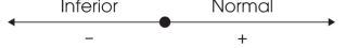
Calculations of this help determine whether the product is inferior or normal good
Inferior good: as income increases, demand for the product decreases
Normal good: as income increases, demand for the product increases
Three Questions to Determine Demand Elasticity
1. Necessity of the product
If the product is a necessity, such as life-saving drugs, prices could increase but people would still purchase it
Products which are wants, such as cars, demand would be price elastic
2. Could the purchase be delayed
The longer the time consumers have the product as a choice, the more elastic the product demand tends to be
If the choice time is limited, the product demand tends to be inelastic
A good example would be emergency supplies
Since the decision time is limited, demand tends to be inelastic
3. Does the purchase require a larger budget range?
If the product forms a large proportion of someone’s budget, demand tends to be elastic
An increase in the price of luxury products would result to consumers stopping their purchase for the time being
On the contrary, products that don’t form a large proportion of someone’s budget such as match sticks, are inelastic in nature (purchased even if prices increases)
Cross-price elasticity of demand
This measures how a demand for a product changes with respect to price changes
Calculations of this help determine whether the product is a complement or substitute
% change quantity demanded for product X/ % change in price of product Y
If the result is positive, the product is substitute
If the result is negative, the product is complement
Price Elasticity of supply
This measures the change in supply that takes place with respect to changes in price
Time is key factor when looking at supply elasticity
The longer the firms have time to adjust, the more elastic the supply (difficult to adjust in the short term hence the inelasticity)
In the longer run, market supply is usually perfectly elastic
% change in quantity supplied / % change in price
If the demand curve is perfectly elastic, there wouldn’t be any consumer surplus
If the supply curve is perfectly elastic, there wouldn’t be any producer surplus
Excise taxes
Per-unit tax on production
Firm responds as if the marginal cost of producing each unit has risen by the amount of the tax
Results in a vertical shift in the supply curve by the amount of the tax
Reason for taxes are:
Increase revenue collected by the government
To decrease consumption of a good that might be harmful to some members of society
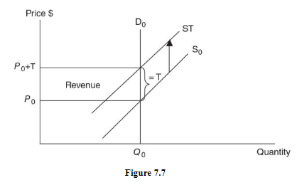
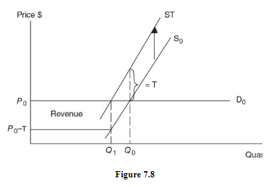
Demand Is Perfectly Inelastic
Assume the following demand is of tobacco
If a per-unit tax of T is imposed on the producers of cigarettes, the supply curve shifts upward by T
Since quantity remained constant, the tax did nothing to decrease the harmful effects of smoking in society
Only increased tax revenues for the government
The entire tax was paid by consumers in the form of a new price exactly equal to the old price plus the tax.
Demand is perfectly elastic
Assume the following demand is of tobacco
The per-unit tax of T shifts the supply curve upward by T
Because the price of a pack of cigarettes did not increase after the tax, it was not the consumers who paid more
Producer pays the entire share of the tax when demand is perfectly elastic
Compared to the perfectly inelastic scenario, the government collected much fewer tax revenue dollars
Maximum decrease in harmful cigarette consumption is a definite plus
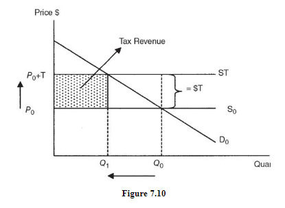
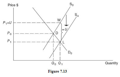
The Role the Supply Curve Plays in the Impact of an Excise Tax
A perfectly elastic, or horizontal, supply curve tells us that even a very small change in the price will cause an infinitely large change in the quantity supplied
The new equilibrium price is exactly T higher than the old price P0, so consumers pay the entire burden of the tax
The equilibrium quantity decreases from Q0 to Q1, and the government collects tax revenue equal to T × Q1.
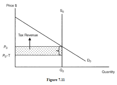
A perfectly inelastic, or vertical, supply curve illustrates the special case where any change in the price creates absolutely no change in the quantity supplied
At the equilibrium quantity Q0, suppliers would like to charge a higher price than P0, but any price above P0 creates a surplus, and this surplus will clear only at the equilibrium price P0.
The firms must pay T to the government for each of the Q0 units that are sold and consumers continue to pay the original price of P0
Producers pay the entire burden of the tax because, after paying the tax, they receive only (P0 – T) on each unit
Price elasticity of supply and tax incidence
Price elasticity of supply | Government revenue | Decrease in consumption | Incidence of tax paid by consumers | Incidence of tax paid by product |
|---|---|---|---|---|
infinity | the least | the most | 100% | 0% |
>1 | falling | sizeable | >50% | <50% |
<1 | rising | minimal | <50% | >50% |
0 | the most | 0 | 0% | 100% |
As the price elasticity of demand falls, and the price elasticity of supply rises, the greater the consumer’s share of a per-unit excise tax
Conversely, as the price elasticity of demand rises and the price elasticity of supply falls, the producer’s share of a per-unit excise tax rises
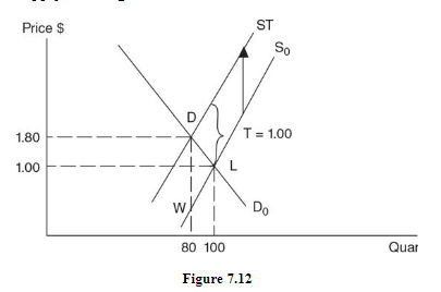
Loss to society
There is also a cost to society when an excise tax is imposed on a competitive market
With the tax, consumers and producers demand and supply 20 fewer units than without the tax
For these 20 units that go unproduced, the marginal benefit to consumers exceeds the marginal costs to producers
20 units go unproduced and unconsumed resulting in an inefficient outcome
Economists call this area deadweight loss (DWL), or the net benefit sacrificed by society when such a per-unit tax is imposed (triangle labeled DWL)
Taxes create lost efficiency by moving away from the equilibrium market quantity where MB = MC to society.
The area of deadweight loss (triangle DWL) increases as the quantity moves further from the competitive market equilibrium quantity
Subsidies
A per-unit subsidy on good X has the opposite effect of an excise tax
Firms respond as if the subsidy has lowered the marginal cost of production
Results in a downward vertical shift in the supply curve for good X
Assume the graph of the market for public university education
The subsidy decreases tuition to P1 and increases the number of undergraduate degrees received
Subsidy distorts the market and creates deadweight loss
Deadweight loss is the area of the triangle labeled DWL.
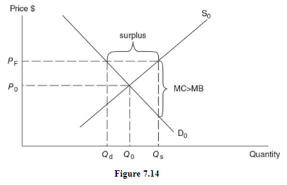
Price Floors
A price floor is a legal minimum price below which the product cannot be sold
An ineffective price floor would be a price set below the equilibrium price
Assume this to be a market for milk
The resulting surplus of milk is not eliminated through the market
The government usually agrees, as part of the price floor arrangement, to purchase the surplus milk
By providing an incentive for producers to produce beyond where MB = MC, the price floor policy causes efficiency to be lost.
For gallons of milk above Q0, MC > MB; there is an over allocation of resources to milk production
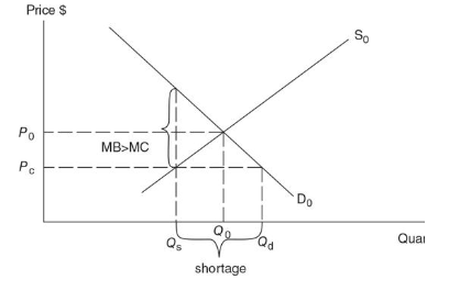
Price Ceilings
A price ceiling is a legal maximum price above which the product cannot be bought and sold
An effective price ceiling must be set below the equilibrium price
Assume this to be a market for rent-controlled households
This form of price control results in lost efficiency for society
When suppliers reduce their quantity supplied below the competitive equilibrium quantity, there is a situation where MB > MC, and we see under allocation of resources in the rental apartment market
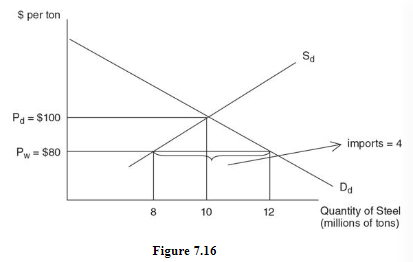
Trade Barriers
1. Tariffs
Revenue tariff is an excise tax levied on goods that are not produced in the domestic market.
Protective tariff is an excise tax levied on a good that is produced in the domestic market
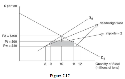
Economic effects of the tariff
Consumers pay higher prices and consume less
Consumer surplus has been lost
Domestic producers increase output
Declining imports
Tariff revenue
Inefficiency
Deadweight loss
2. Quotas
Import quota is a maximum amount of a good that can be imported into the domestic market
Both hurt consumers with artificially high prices and lower consumer surplus.
Both protect inefficient domestic producers at the expense of efficient foreign firms, creating a deadweight loss.
Both reallocate economic resources toward inefficient producers.
Tariffs collect revenue for the government, while quotas do not
Consumer Choice
Utility
People demand things because those things make those people happy
In economics, we call this happiness utility
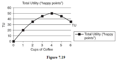
Consumption of more and more of something is likely to increase our total utility
It is probably safe to say that the first pint in a week provides more marginal utility than the second, third, or fourth pint
Total utility (TU) is the total amount of happiness received from the consumption of a certain amount of good.
Marginal utility (MU) is the additional utility received from the consumption of the next unit of a good
MU = ∆TU/∆Q
Unconstrained consumer choice
Total utility initially rises, peaks, and then begins to fall as more coffee is consumed(see fig above)
Even if the monetary price of good X is zero, the rational consumer stops consuming good X at the point where total utility is maximized.
Diminishing marginal utility
The law of diminishing marginal utility says that in a given time period, the marginal utility from consumption of one more of that item falls
Constrained utility maximization
With a fixed daily income and a price that must be paid, this individual is now a constrained utility maximizer
When required to pay a price, the utility-maximizing consumer stops consuming when MB = P.
This MB also represents the highest price, or “willingness to pay,” our consumer would be willing to pay for the next cup.
Demand curve revisited
Law of diminishing marginal utility is the backbone of the law of demand
Because of diminishing marginal utility, you offer to pay less for additional units
Utility maximizing rule
Consumers maximize utility when they buy amounts of goods X and Y so that the marginal utility per dollar spent is equal for both goods
MUx/Px = MUy/Py
If the consumer has used all income and the above ratios are equal, they are said to be in equilibrium
It is very important to remember that consuming more of one good causes the marginal utility to fall, but the total utility to rise
To find the total utility of consuming cups of coffee, sum up the marginal utility of each cup consumed. Do the same for scones to calculate total utility
Cups of coffee | MU of coffee | # of Scones | MU of Scone |
|---|---|---|---|
1 | 10 | 1 | 30 |
2 | 8 | 2 | 24 |
3 | 6 | 3 | 20 |
4 | 4 | 4 | 16 |
5 | 2 | 5 | 14 |
6 | 1 | 6 | 8 |
MUc/MUs = $2/$4= .5 or
MUc/MUs = $1/$4 = .25