Membrane Potential Assignment

• Membrane potential: The separation of charge across a membrane, measured in mV

• Ungated channels (Na+, K+) are always open

  • Na+ channels flow in

  • K+ channels flow out

• Na+/K+ Exchange Pump is active, going against the gradient, keeping unequilibrium and net negative charge.

  • 3 Na+ out, 2 K+ in

• Neuronal Excitation: The firing of an action potential down the axon, caused by rapid redistribution of ions across the axonal plasma membrane.

  • Redistribution reverses electrical charge across the membrane, causing a membrane potential.

    • Membrane potential goes from around -65 mV to +40 mV.

• Membrane proteins are amphipathic (part hydrophilic, part hydrophobic) to be able to work well with the tails, but also water/ions.

• Facilitated diffusion needs no additional energy, ions pass through channels down their electrochemical gradient, which is determined by the charge of the ion as well as the concentration of the ion on each side of the membrane.

• Equilibrium Potentials: The membrane potential at which diffusional and electrical forces on an ion are equal and opposite. When equilibrium potential is reached, there is no further net movement of the ions.

• Calculating Eion, The Nernst Equation

  • Eion = 2.303(RT/zF) x log[ion]outside/[ion]inside

  • OR

  • Eion = RT/zF x ln [ion]outside/[ion]inside

    • R = 8.314 J/K*mol

    • T = Temp in K (body temp = 37 degrees C or 310 K)

    • z = Charge on the ion

    • F = 9.648 x 10^4 C/mol

• What keeps Na+, K+, and Ca2+ from reaching equilibrium?

  • The neuronal plasma membrane is differentially permeable to ions (more ungated K+ than ungated Na+ channels).

  • K+ crosses more readily.

• The Na+/K+ pump maintains an imbalance of Na+ and K+ across the membrane.

  • ATP dependent

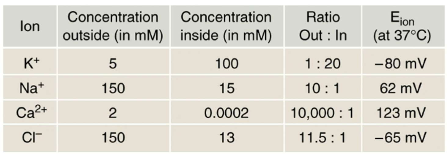
• Typical concentrations inside and outside the neuron

  • K+

    • Outside: 5 mM

    • Inside: 100 mM

  • Na+

    • Outside: 150 mM

    • Inside: 15 mM

  • Ca2+

    • Outside: 2 mM

    • Inside: 0.2 microM

  • Cl-

    • Outside: 150 mM

    • Inside: 13 mM

• Rate of ion movement, Ionic Driving Force

  • Ionic driving force = |Vm - Eion|

    • Always positive

• The Goldman Equation

  • Vm = RT/F * ln (pK+[K+]o + pNa+[Na+]o + pCl-[Cl-]i) / (pK+[K+]i + pNa+[Na+]i + pCl-[Cl-]o)

    • pK+ = 2.84 x 10^-8 m/sec

    • pNa+ = 6.85 x 10^-10 m/sec

    • pCl- = 0 m/sec

Part 1: Acetylcholinesterase Assay (Week 1)

• Objective: To determine which region of the brain (frontal cortex, striatum, hippocampus, and cerebellum) has the highest amounts of ACh.

• Testing 4 regions of the brain: Frontal Cortex, Striatum, Hippocampus, and Cerebellum

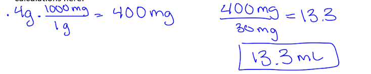
• The brain is homogenized with 0.1 M Phosphate Buffer (PB) to produce a 30 mg (homogenate)/ml (PB) solution.

  • Homogenized using a sonicator, which uses sound waves to break apart tissue.

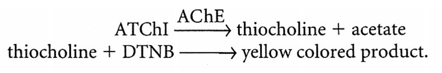
• Brain homogenate is the source of AChE (the enzyme) that breaks down ATChI into acetate and choline

• Ellman Assay (above) quantifies the amount of ATChI broken down by the enzyme in the brain homogenate to determine which brain region of the 4 tested has the highest amounts of AChE/ACh.

• Be able to calculate the volume of 0.1 M PB needed to produce a 30mg/ml homogenate.

• After sonicating, place the homogenate on ice.

• Materials

  • Brain homogenate (source of enzyme)

  • 0.1 M Phosphate Buffer (PB)

  • 0.01 M DTNB (interacts with thiocholine to produce the yellow-colored product and acetate)

  • 0.075 M ATChI (Acetylcholine Iodide, the substrate that forms thiochlorine as a product)

  • Spectrophotometer set to a wavelength of 412 nm

  • Test tube rack containing 4 test tubes, labeled “Con, 1, 2, and 3”, each filled with 3 mL 0.1 M PB.

Performing the Ellman Assay

1. Add 200 microliters of the brain homogenate (enzyme) to each tube, cover with parafilm, vortex, and place on ice.

2. Add 100 microliters of 0.01 M DTMB to each tube, vortex, and place at room temperature for 5 min.

3. Place the “con” tube in the spectrophotometer and zero it as your negative control sample.

4. Remove the sample tube, quickly add 20 microliters of 0.01 M PB, cover with a gloved finger, invert once, and immediately return to the spectrophotometer. Read the absorbance values at 30-second intervals for 3 minutes.

5. For tubes 1-3, quickly add 20 microliters of 0.075 M ATChI instead of PB, cover with a gloved finger, invert once, and immediately return to the spectrophotometer. Read the absorbance values at 30-second intervals for 3 minutes.

Calculations and Graphing

• The rate being determined will be the amount of ATChI that is broken down by AChE per minute.

• Calculate the rate of product formation per minute by adding a linear trendline to each data set on the graph and showing the equation of each line on the graph. The equation will tell you the slope, which is the change in absorbance over time. Then calculate the mean rate of product formation for all 3 trials.

• Calculate the reaction rate in micromoles of substrate hydrolyzed/min * gram of tissue

  • Determine by using the equation: R = 1220 * (mean slope)/0.03

  • The reaction rate determines which region has the highest rate of AChE activity, and therefore the highest amount of ACh

    • Supposed to be Striatum

Part 2: AChE Inhibition Assay (Week 2)

• Objective: To determine if tacrine is a competitive or non-competitive inhibitor of AChE.

• Materials

  • Brain homogenate on ice (source of enzyme), whole brain

  • 0.1 M phosphate buffer (PB)

  • 0.01 M DTMB

  • Tacrine on ice (source of inhibitor)

  • 6 different aliquots of ATChI on ice (substrate)

    • 0.01 M

    • 0.02 M

    • 0.04 M

    • 0.06 M

    • 0.08 M

    • 0.1 M

  • 14 test tubes, each filled with 3 mL of 0.01 M PB

    • 1-7 differing concentrations of ATChI w/out Tac (uninhibited reactions)

    • 8-14 differing concentrations of ATChI w/ Tac (inhibited reactions)

    • Spectrophotometer set to a wavelength of 412 nm

Performing the Assay

1. Add 200 microliters of the brain homogenate to each of the inhibited reaction tubes (#8-14), cover with parafilm, vortex, and place on ice.

2. Add 40 microliters of the inhibitor to each of the inhibited reaction tubes (#8-14), and let sit on ice until you have finished the assay on the uninhibited reaction tubes.

3. Add 200 microliters of the brain homogenate to each of the uninhibited reaction tubes (#1-7), cover with parafilm, vortex, and place on ice.

4. Add 100 microliters of 0.01 M DTMB to each tube, vortex, and place at room temperature for 5 min.

5. Place the “con” tube in the spectrophotometer and zero it as your negative control sample.

6. Remove the sample tube, quickly add 20 microliters of 0.01 M PB, cover with a gloved finger, invert once, and immediately return to the spectrophotometer. Read the absorbance values at 30-second intervals for 3 minutes.

7. For tubes 2-7, quickly add 20 microliters of differing concentrations ATChI instead of PB, cover with a gloved finger, invert once, and immediately return to the spectrophotometer. Read the absorbance values at 30-second intervals for 3 minutes.

Inhibited samples

8. Add 100 microliters of 0.01 M DTNB to each tube of the inhibited samples (#8-14), vortex and place at room temperature for 5 mins.

9. Place the “con” tube in the spectrophotometer and zero it as your negative control sample.

10. Remove the sample tube, quickly add 20 microliters of 0.01 M PB, cover with a gloved finger, invert once, and immediately return to the spectrophotometer. Read the absorbance values at 30-second intervals for 3 minutes.

11. For tubes 9-14, quickly add 20 microliters of differing concentrations ATChI instead of PB, cover with a gloved finger, invert once, and immediately return to the spectrophotometer. Read the absorbance values at 30-second intervals for 3 minutes.

Calculations and Graphing:

Michaelis-Menten Plots

• Figure 3 shows absorbance as a function of time for the uninhibited reactions and should have 7 trendlines, with equations of the line shown on the graph.

• Figure 4 shows absorbance as a function of time for the inhibited reactions and should have 7 trendlines, with equations of the line shown on the graph.

• Convert the slope of each of the lines on both graphs to a rate of moles of ATChI hydrolyzed/min x gram tissue using the R= 1220 * ΔA/0.03 equation.

• Graph the data, the graph will have 2 lines, one for uninhibited reactions and one for inhibited reactions. These are your Michaelis-Menten plots.

Lineweaver-Burk Plots

• Convert your substrate concentration values and reaction rates to their reciprocal values to generate the Lineweaver-Burk plots.

• Plot as a scatter graph with unconnected dots and add linear trendlines to each data set, showing the equation of each line on the graph. You will have to extend your axes and trendlines into the negative quadrants to be able to see where each line crosses the x-axis.

• From the equations of the line, you can now calculate the Vmax and Km for the uninhibited and inhibited reactions.

  • Y-intercept = 1/Vmax

  • X-intercept = -1/Km

• Tacrine is a non-competitive inhibitor